Download
1 / 18
180 likes | 304 Views
Limits of static processing in a dynamic environment. Matt King, Newcastle University, UK. Static Processing. Good for these examples. Static Processing. But what about this?. Detrended. 5 min positions. Whillans Ice Stream. Background. Common GPS processing approaches in glaciology

E N D
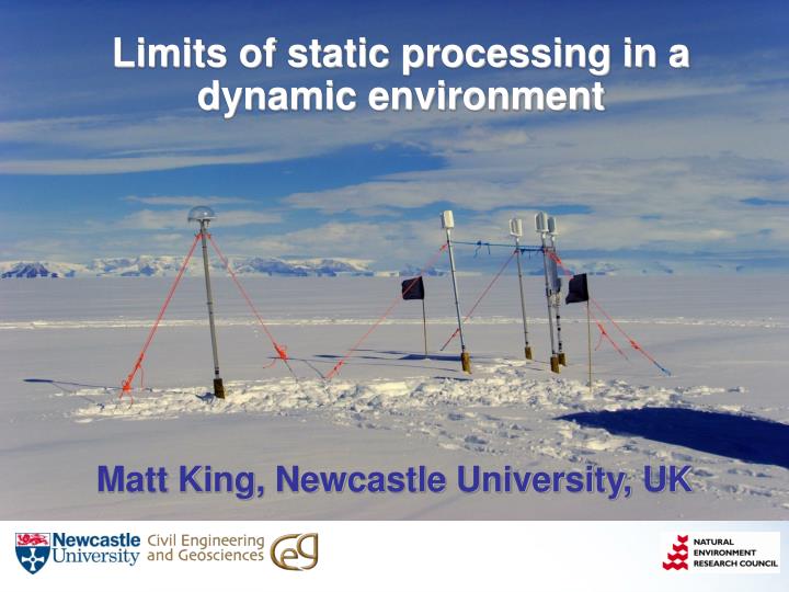
Limits of static processing in a dynamic environment Matt King, Newcastle University, UK
Static Processing • Good for these examples
Static Processing • But what about this? Detrended 5 minpositions Whillans Ice Stream
Background • Common GPS processing approaches in glaciology • Kinematic approach • Antenna assumed moving constantly • Coordinates at each and every measurement epoch • Kinematic solutions often difficult due to long between-site differences • Quasi-static approach • Antenna assumed stationary for certain periods (~0.5-24h) • 24h common for solid earth • <4h common for glaciology • But is this always valid?
GPS Data Processing Approaches • Quasi-static • Kinematic • Quasi-static assumption is that site motion during each session is “averaged out” ~0.5-24h White noise or random walk model
Motion and Least Squares • Functional model • Should fully describe the relationship between parameters X and observation lwithnormally distributed residualsv F(X)=l + v • Stochastic model • Can attempt to mitigate or account for functional model deficiencies • Unmodelled (i.e., systematic) errors will propagate according to the geometry of the solution • Station-satellite geometry • Estimated parameters (e.g., undifferenced “Precise Point Positioning” solutions vs double-differenced; ambiguity fixed vs ambiguity float)
Systematic Error Propagation • Estimated parameters • Station coordinates (X,Y,Z) • AND real-valued phase ambiguity (N) parameters • Clock errors differenced out (in double difference solutions) • Once ambiguities estimated, statistical tests applied to fix to integers • Fixing not always possible • Site motion could induce incorrect ambiguity fixing
Real vs Imaginary:Example on the Amery Ice Shelf GAMIT 1hr quasi-static solutions Track Kinematic solution King et al., J Geodesy, 2003
What’s happening? • Presence of motion during ‘static’ sections • Violates least-squares principle of normal residuals • Leads to biased parameter estimates • Simulation • How does a ~1m/day signal and ~1m tidal signal in 1 hr ‘static’ solutions propagate into the parameters? • Real broadcast GPS orbits • Precise Point Positioning approach simulated • Site ~70S
Ambiguity estimates mapped What’s happening? Latitude North (m) Ambiguities fixed East (m) Height (m) Ambiguities not fixed Satellites East of site Ambiguity (m)
Horizontal Motion Only • GAMIT 1h solutions over modified “zero” baseline Period related to satellite pass time? ~0°N ~90°S
Horizontal Motion Only • Simulation – grounded case • How does a ~1m/day signal 1 hr ‘static’ solutions propagate into the parameters? • Various flow directions (N, NE, E) • 1hr solutions • Various latitudes • Site ~70S
What’s Happening? Ambiguity estimates mapped North (m) Ambiguities fixed Ambiguities not fixed East (m) Height (m) King et al., J Glac., 2004
Whillans Ice Stream • Based on simulation would expect • Agreement during ‘stick’ • Biases during ‘slip’ • But not in kinematic solutions 4hr quasi-static solutions 5min kinematic solutions
Solid Earth Issues • Propagation of mis/un-modelled periodic signals (e.g., ocean tide loading displacements) in 24h solutions • Well described by Penna & Stewart (GRL, 2003) and Penna et al., JGR, 2007. • Admittances in float ambiguity PPP solutions >120% in worst case (S2 north component into local up) • Depends on coordinate component of mismodelled signal & frequency & “geometry” • Output frequencies depend on input frequency • Annual, semi-annual and fortnightly, amongst many others
Periodic Signals mm Penna et al., JGR, 2007
Effect in real data • King et al, GRL, 2008
Conclusions • Biases may exist in positions on moving ice from GPS • Up to 40-50% of unmodelled vertical signal • Up to ~10% of unmodelled horizontal signal • May be offsets, periodic signals or both in east, north and height components • Height biases of concern when validating Lidar missions • Periodic signals may result in wrong interpretation as tidal modulation (or contaminate real tidal modulation) • To measure bias-free ice motion using GPS • Fix ambiguities to correct integers (not always possible) • Use kinematic solution (may require non-commercial software) • For 24h solutions • Periodic signals propagate • Other sub-daily signals (e.g., multipath) need further study