Download
1 / 54
580 likes | 1.13k Views
Confounding and Interaction: Part III. Methods to reduce confounding during study design : Randomization Restriction Matching during study analysis: Stratified analysis Forming “Adjusted” Summary Estimates Concept of weighted average Woolf’s Method Mantel-Haenszel Method

E N D
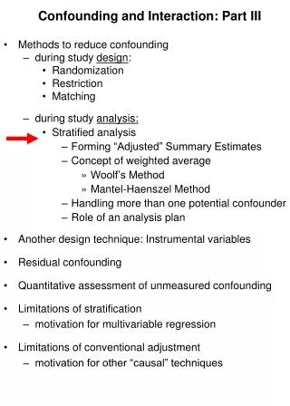
Confounding and Interaction: Part III • Methods to reduce confounding • during study design: • Randomization • Restriction • Matching • during study analysis: • Stratified analysis • Forming “Adjusted” Summary Estimates • Concept of weighted average • Woolf’s Method • Mantel-Haenszel Method • Handling more than one potential confounder • Role of an analysis plan • Another design technique: Instrumental variables • Residual confounding • Quantitative assessment of unmeasured confounding • Limitations of stratification • motivation for multivariable regression • Limitations of conventional adjustment • motivation for other “causal” techniques
Effect-Measure Modification Crude RR crude= 1.7 Heavy Caffeine Use No Caffeine Use Stratified RRcaffeine use = 0.7 RRnocaffeine use = 2.4 . cs delayed smoking, by(caffeine) caffeine | RR [95% Conf. Interval] M-H Weight -----------------+------------------------------------------------- no caffeine | 2.414614 1.42165 4.10112 5.486943 heavy caffeine | .70163 .3493615 1.409099 8.156069 -----------------+------------------------------------------------- Crude | 1.699096 1.114485 2.590369 M-H combined | 1.390557 .9246598 2.091201 -----------------+------------------------------------------------- Test of homogeneity (M-H) chi2(1) = 7.866 Pr>chi2 = 0.0050 Report interaction; confounding is not relevant (but it has been managed)
Report vs Ignore Effect-Measure Modification?Some Guidelines Is an art form: requires consideration of clinical, statistical and practical considerations P value threshold might be higher but interpretation is no different
Does AZT after needlesticks prevent HIV? Crude ORcrude =0.61 Stratified Minor Severity Major Severity OR = 0.35 OR = 0.0 Report or ignore interaction?
General Framework for Stratification • Design phase: Create a DAG • Decide which variables to control for • Implementation phase: measure the confounders (or other variables needed to block path) and potential effect modifiers • Analysis phase: Form Strata Report Effect-Measure Modification? (assess clinical, statistical, and practical considerations) Report stratum-specific estimates no yes Derive summary “adjusted” estimate + Decide which variables, if any, to adjust for to derive final estimate none some Report crude estimate, 95% CI, p value Report adjusted estimate, 95% CI, p value (Things get complicated with > 1 extra variable)
What Next? Crude ORcrude = 0.61 Stratified Minor Severity Major Severity OR = 0.0 OR = 0.35 How would you summarize these strata into one number?
Assuming Interaction is not Present, Form a Summary of the Unconfounded Stratum-Specific Estimates • Construct a weighted average • Assign weights to the individual strata • Summary Adjusted Estimate = Weighted Average of the stratum-specific estimates • a simple mean is a weighted average where the weights are equal to 1 • which weights to use depends on type of effect estimate desired (OR, RR, RD), characteristics of the data, and goal of research • e.g., • Woolf’s method • Mantel-Haenszel method • Standardization (see text) • Discussed earlier for age adjustment
Forming a Summary Adjusted Estimate for Stratified Data Crude ORcrude = 0.61 Stratified Minor Severity Major Severity OR = 0.0 OR = 0.35 How would you weight these strata?
Summary Estimators: Woolf’s Method • aka Directly pooled or precision estimator • Woolf’s estimate for adjusted odds ratio • where wi • wi is the inverse of the variance of the stratum-specific log(odds ratio)
Calculating a Summary Effect Using the Woolf Estimator • e.g., AZT use, severity of needlestick, and HIV Crude ORcrude =0.61 Stratified Minor Severity Major Severity OR = 0.0 OR = 0.35 Problem: cannot take log of 0; cannot divide by zero
Summary Adjusted Estimator: Woolf’s Method • Conceptually straightforward • Best when: • number of strata is small • sample size within each stratum is large • Cannot be calculated when any cell in any stratum is zero because log(0) is undefined • “1/2” cell corrections have been suggested but are subject to bias • Formulae for Woolf’s summary estimates for other measures (e.g., risk ratio, RD) available in texts and software documentation • Rarely used in practice but most clearly illustrates weighting
Summary Adjusted Estimators: Mantel-Haenszel • Mantel-Haenszel estimate for odds ratios • ORMH = • wi = • wi is inverse of the variance of the stratum-specific odds ratio under the null hypothesis (OR =1)
Summary Adjusted Estimator: Mantel-Haenszel • Relatively resistant to the effects of large numbers of strata with few observations • Resistant to cells with a value of “0” • Computationally easy • Most commonly used in commercial software
Calculating a Summary Adjusted Effect Using the Mantel-Haenszel Estimator • ORMH = • ORMH = Crude ORcrude =0.61 Stratified Minor Severity Major Severity OR = 0.0 OR = 0.35
Calculating a Summary Effect in Stata • To stratify by a third variable: • cs varcase varexposed, by(varthird variable) • cc varcase varexposed, by(varthird variable) • Default summary estimator is Mantel-Haenszel • “ , pool” will also produce Woolf’s method • To stratify by several variables: • mhodds varcase varexposed varsadjust, by(varsstratify) • Problem set this week epitab command - Tables for epidemiologists A good place to learn epidemiology
Calculating a Summary Effect Using the Mantel-Haenszel Estimator • e.g. AZT use, severity of needlestick, and HIV • . cc HIV AZTuse,by(severity) pool • severity | OR [95% Conf. Interval] M-H Weight • -----------------+------------------------------------------------- • minor | 0 0 2.302373 1.070588 • major | .35 .1344565 .9144599 6.956522 • -----------------+------------------------------------------------- • Crude | .6074729 .2638181 1.401432 • Pooled (direct) | . . . • M-H combined | .30332 .1158571 .7941072 • -----------------+------------------------------------------------- • Test of homogeneity (B-D) chi2(1) = 0.60 Pr>chi2 = 0.4400 • Test that combined OR = 1: • Mantel-Haenszel chi2(1) = 6.06 • Pr>chi2 = 0.0138 Crude ORcrude =0.61 Stratified Minor Severity Major Severity OR = 0.0 OR = 0.35
Calculating a Summary Effect Using the Mantel-Haenszel Estimator • In addition to the odds ratio, Mantel-Haenszel estimators are also available in Stata for: • risk ratio/prevalence ratio • “cs varcase varexposed, by(varthird variable)” • rate ratio • “ir varcase varexposed vartime, by(varthird variable)”
After Confounding is Managed: Confidence Interval Estimation and Hypothesis Testing for the Mantel-Haenszel Estimator • e.g. AZT use, severity of needlestick, and HIV • . cc HIV AZTuse,by(severity) pool • severity | OR [95% Conf. Interval] M-H Weight • -----------------+------------------------------------------------- • minor | 0 0 2.302373 1.070588 • major | .35 .1344565 .9144599 6.956522 • -----------------+------------------------------------------------- • Crude | .6074729 .2638181 1.401432 • Pooled (direct) | . . . M-H combined | .30332 .1158571 .7941072 • -----------------+------------------------------------------------- • Test of homogeneity (B-D) chi2(1) = 0.60 Pr>chi2 = 0.4400 • Test that combined OR = 1: • Mantel-Haenszel chi2(1) = 6.06 • Pr>chi2 = 0.0138 • What does the p value = 0.0138 mean?
Terminology • “Use of AZT is associated with decreased odds of HIV acquisition, independent of needlestick severity” • “Use of AZT is associated with decreased odds of HIV acquisition, adjusted for needlestick severity” • “Use of AZT is associated with decreased odds of HIV acquisition, controlling for needlestick severity” • “Use of AZT is associated with decreased odds of HIV acquisition, conditioned on needlestick severity”
Independence • “Use of AZT is associated with decreased odds of HIV acquisition, independent of needlestick severity” • “independent of” simply refers to adjustment/control for other factors • Does not refer to whether or not adjusted estimate is different from crude • Just means that adjustment has been performed (e.g., via stratification) and there remains (or does not remain) an association between exposure and disease
How about this? • “Use of AZT is causally related to reduced HIV acquisition.” • Formally, our analyses produce statistical associations, which could have resulted from: • Causal relationship (Truth) Or bias due to: • Selection bias • Measurement bias • Confounding bias Or • Reverse causality (but not here) Or • Chance • A single observational study rarely proves causality
Mantel-Haenszel Techniques • Mantel-Haenszel estimators • Mantel-Haenszel chi-square statistic • Mantel’s test for trend (dose-response)
Spermicides, maternal age & Down Syndrome Crude OR = 3.5 Age < 35 Age > 35 Stratified OR = 3.4 OR = 5.7 Which answer should you report as “final”? What undesired feature has stratification caused?
Effect of Adjustment on Precision (Variance) • Adjustment can increase or decrease standard errors (and CI’s) depending upon: • Nature of outcome (interval scale vs. binary) • Measure of association desired • Method of adjustment (Woolf vs M-H vs MLE) • Strength of association between potential confounding factor and exposure/disease • Complex and difficult to predict • Good news: adjustment for strong confounders removes bias and often improves precision • Bad news: adjustment for less-than-strong confounders can often (but not always) worsen precision
Effect of Adjustment on Precision Crude ORcrude = 21.0 (95% CI: 16.4 - 26.9) Stratified Matches Present Matches Absent ORmatches = 21.0 OR nomatches = 21.0 ORadj= 21.0 (95% CI: 14.2 - 31.1) Avoid this by not adjusting for factors unless they are on your DAG
Spermicides, maternal age & Down Syndrome Crude OR = 3.5 Age < 35 Age > 35 Stratified OR = 3.4 OR = 5.7 Which answer should you report as “final”?
Whether or not to accept the “adjusted” summary estimate instead of the crude? • Methodologic literature is inconsistent on this • Bias-variance tradeoff • Scientifically most rigorous approach is to: • Create the DAG and identify potential confounders • Prior to adjustment, classify the potential confounders as either being: • “A” List: Those factors for which you will accept the adjusted result no matter how small the difference from the crude. • Factors strongly believed to be confounders • “B” List: Those factors for which you will accept the adjusted result only if it meaningfully differs from the crude (with some pre-specified difference, e.g., 5 to 10%). • Factors you are less sure about • “Change-in-estimate” approach • For some analyses, may have no factors on A list. For other analyses, no factors on B list. • Always putting all factors on A list may seem “conservative”, but not necessarily the right thing to do in light of penalty of statistical imprecision Bias control paramount Need for tradeoffs
Choosing the crude or adjusted estimate? • Assume no interaction • Factors on B list have 10% change-in-estimate rule in place
No Role for Statistical Testing for Confounding • Testing for statistically significant differences between crude and adjusted measures is inappropriate • e.g., examining an association for which a factor is a known confounder (say age in the association between hypertension and CAD) • if the study has a small sample size, even large differences between crude and adjusted measures may not be statistically different • yet, we know confounding is present • therefore, the difference between crude and adjusted measures cannot be ignored as merely chance. • bias must be prevented and hence adjusted estimate is preferred • we must live with whatever effects we see after adjustment for a factor for which there is a strong a priori belief about confounding • If study has large sample size, even small differences between crude and adjusted will be significant. Would you accept all of these adjustments to be necessary even if no a priori evidence of confounding?
No Role for Statistical Testing for Confounding • Subject matter knowledge trumps statistical testing
Spermicides, maternal age & Down Syndrome Crude OR = 3.5 Age < 35 Age > 35 Stratified OR = 3.4 OR = 5.7 Which answer should you report as “final”? Either is OK, depending upon your analysis plan
Stratifying by Multiple Potential Confounders Crude Stratified <40 smokers 40-60 smokers >60 smokers <40 non-smokers 40-60 non-smokers >60 non-smokers Adjust for these 2 factors jointly or one-by-one?
The Need for Evaluation of Joint Confounding • Variables that evaluated alone show no confounding may show confounding when evaluated jointly Crude Stratified by Factor 1 alone by Factor 2 alone by Factor 1 & 2
WHO Causal Model of Coronary Heart Disease Murray et al. Population Health Metrics 2003
Approaches for When More than One Potential Confounder is Present • Backward vs forward variable selection strategies • relevant both for stratification and multivariable regression modeling (“model selection”) • Backwards Strategy • initially evaluate all potential confounders together (i.e., look for joint confounding) • preferred because in nature variables act together • Procedure: • with all potential confounders considered (A+B), form adjusted estimate. This is “gold standard” • Of variables on the B list, one variable can then be dropped and the adjusted estimate is re-calculated (adjusted for remaining variables) • if the dropping of the first variable results in non-meaningful (eg < 5 or 10%) change compared to the gold standard, it can be eliminated • “change-in-estimate” approach • continue until no more variables can be dropped (i.e. all remaining variables are relevant) • Problem: • With too many potential confounders, cells become very sparse in stratification or “overfitting” occurs in regression
Approaches for When More than One Potential Confounder is Present • Forward Strategy • start with the variable that has the biggest “change-in-estimate” impact (adjusted vs crude) when evaluated individually • then add the variable with the second biggest impact • keep this variable if its presence meaningfully changes the adjusted estimate (e.g., >5 or >10%) • procedure continues until no other added variable has an important impact • Advantage: • avoids the initial sparse cell problem of backwards approach • Problem: • does not evaluate joint confounding effects of many variables
An Analysis Plan • How to select final variables to control for (final set) is one of the least standardized processes in clinical research • Available methods often arbitrary and can give different answers for the “final estimate” • Invites fishing for desired answers • Solution: Analysis plan • Written before the data are analyzed • Content • Detailed description of the techniques to be used to analyze data, step by step • Forms the basis of “Statistical Analysis” section in manuscripts • Parameters/rules/logic to guide key decisions: • which variables will be assessed for interaction and for adjustment? • what p value and magnitude of heterogeneity will be used to guide reporting of interaction? • what is a meaningful change-in-estimate threshold between two estimates (e.g., 10%) to determine variable selection? • Utility: A plan helps to keep the analysis: • Focused • Transparent • Reproducible • Honest (avoids p value shopping)
Transparency of Analytic Plans • Poor Quality of Reporting Confounding Bias in Observational: A Systematic Review. Groenwold et al. Ann Epid 2008 • Review of 174observational studies, 2004 - 2007
Final Advice for Variable Selection • Many approaches • Will learn about in Biostat II and III • No single best approach • Researchers tend to develop own style • Our advice • Be transparent • Have an analysis plan • Remember: • Variables operate jointly in nature • The motivation, which is to manage confounding bias • Hence, tend towards bias control in the bias-variance tradeoff
Hour of birth Length of stay Unmeasured C Prenatal complications ? Neonatal outcomes Instrumental Variables to Manage Confounding Instrumental variable (IV) IV must be related to E but nothing else E Unmeasured C C1 C2 ? D Use IV—D and IV—E associations to estimate unconfounded E—D RQ: Does length of stay determine neonatal outcomes? Malkin et al. Heath Serv. Res., 2000
Residual Confounding Four Mechanisms • Categorization of confounder too broad • e.g., Association between natural menopause and prevalent CHD Szklo and Nieto, 2007 • Misclassification of confounders • Can be differential or non-differential with respect to exposure and disease • If non-differential, will lead to adjusted estimates somewhere in between crude and true adjusted • If differential, can lead to a variety of unpredictable directions of bias
Periodontal disease E Inflammatory Predisposition Unmeasured C Age CRP level ? ? CAD D Residual Confounding Mechanisms – cont’d • Variable used for adjustment is imperfect surrogate for true confounder • Unmeasured confounders
Quantitative Analysis of Unmeasured Confounding • Can back calculate to determine how a confounder would need to act in order to spuriously cause any apparent odds ratio. Example: observed OR= 2.0 Prevalence of “high” level of unmeasured confounder Association between unmeasured confounder and exposure (prevalence ratio) Association between unmeasured confounder and disease (risk ratio) A (low prevalence scenario) = 7 B (high prevalence scenario) = 3.4 Winkelstein et al., AJE 1984
Quantitative assessment of unmeasured confounders • “The contour plot shows that a confounding factor with a relative risk for death of 4.0 and an odds ratio for deferral of therapy of 4.0 after adjustment for all included variables would reduce the estimated relative risk for deferred therapy to approximately 1.30.” Kitahata et al. NEJM 2009
Quantitative Bias Analysis • Our discussion of selection, measurement, and confounding bias has been qualitative • Frontier of epidemiologic methods is quantitative bias analysis • Selection bias: use estimates of selection probabilities to back-calculate to truth • Measurement bias: use estimates of misclassification to back-calculate to truth • Confounding: How would results change in presence of certain confounding factors?
Stratification to Manage Confounding • Advantages • straightforward to implement and comprehend • easy way to evaluate interaction • Limitations • Requires continuous variables to be discretized • loses information; possibly results in “residual confounding” • discretizing often brings less precision • Deteriorates with multiple confounders • e.g., suppose 4 confounders with 3 levels • 3x3x3x3=81 strata needed • unless huge sample, many cells have “0”’s and strata have undefined effect measures • Conventional Solution: • Mathematical modeling (multivariable regression) • e.g. • linear regression • logistic regression • proportional hazards regression
Limitation of Conventional Stratification (and Regression) • Scenario: Time-varying exposures in the presence of time-varying confounders/mediators • e.g., Cohort study of effect of antiretroviral therapy (ART) on AIDS incidence ART- time 1 ART- time 2 ? CD4 count or viral load Severity of HIV (unmeasured) AIDS Simultaneous desire to control for CD4/viral load to manage confounding and but NOT to control because it is a collider
When factors are simultaneously confounders and mediators, conventional techniques fail and other “causal methods” are needed Causal methods: g-estimation; structural nested models; and marginal structural models (inverse probability weighting) Cole et al, AJE 2003
Limitation of Conventional Stratification (and Regression) • Scenario: Determining a direct effect • e.g., Direct effect of E on D apart from effect on M and X E ? X M D Unmeasured Confounder Simultaneous desire to control for M and X to get direct effect of E and but NOT to control because they are colliders Other causal methods needed