Download
1 / 32
320 likes | 514 Views
Chapter 12 Lot Streaming Procedures for the Flow Shop. 2013 년 2 학기 스케줄이론 (406.653) Prof. Jinwoo Park. Contents. 1. Introduction 2. The Basic Two Machine Model 2.1 Preliminaries 2.2. The Continuous Version 2.3. The Discrete Version

E N D
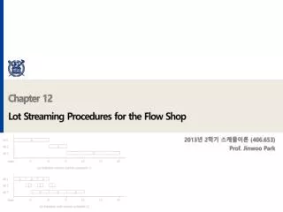
Chapter 12Lot Streaming Procedures for the Flow Shop 2013년 2학기 스케줄이론(406.653) Prof. Jinwoo Park
Contents 1. Introduction 2. The Basic Two Machine Model 2.1 Preliminaries 2.2. The Continuous Version 2.3. The Discrete Version 3. The Three-Machine Model with Consistent Sublots 3.1. The Continuous Version 3.2. The Discrete Version 4. The Three-Machine Model with Variable Sublots 4.1. Item and Batch Availability 4.2. The Continuous Version 4.3. The Discrete Version 4.4. Computational Experiments 5. The m-Machine Model with Consistent Sublots 5.1. The Two SublotSolution 5.2. An s-Sublot Heuristic Procedure 6. Summary 1 2 3 4 5 6
Introduction • Splitting a lot arises in two cases: • Preemption (due to priorities) • Lot Streaming (to move fast) • DefinitionProcess batch vs. Transfer batch
Terminology • : Lot size (of the same items) • : The processing time per unit at machine i • : The size of the jthsublot on machine i (j=1,…,s) and • Called a discrete lot streaming problem if s are integers • Let , then • If , then we call the sublots consistent (otherwise, we have variable sublots)
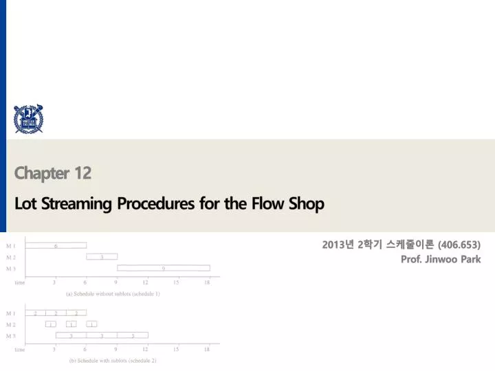
Example Five machine, processing time 5,9,4,7,6, production lot size 100 Ordinarily 3100, but with Lot Streaming, can be finished in 2000 FIGURE 12.1 A solution to Example 12.1 with two equal sublots
The Basic Two Machine Model - Preliminaries • The makespan if done by one lot • For two machine cases, "consistent sublots" and "no idling" do not affect performance. Dominance Relationships There is no dominance relationship among consistency and idling, but the most optimum solution is obtained when there is no restriction on consistency and idling.
The Continuous Version • Rescale the problem so that • Let us focus out attention on sublot k so that (k-1) sublots on machine 1, and (s-k) sublots on machine 2. • Now • When k=1, , and k=s, • Equality must hold for (1) for at least one k • We call such sublot c as “critical sublot”
The Continuous Version . Theorem 12.1 In the optimal solution for a two-machine lot streaming problem, all sublots are critical. • Proof • When critical sublot has slack • When non-critical sublot has slack • From the Theorem, we induce that the successive sublots satisfy the relation • And in the original scale, we obtain
The Discrete Version • Naive round-off of solutions obtained by continuous version may not work(rounding off will move sublot sizes in the same direction. We need a little bit sophisticated method for rounding off. • Try out for the given makespan M, and if infeasible increase the makespan M until we get feasible solution (we have a polynomial time algorithm). • Let denote the cumulative number of items in the first j sublots, ie • Assuming M be the makespan, the last start time for the jthsublot on machine 2 is
The Discrete Version • For feasibility, we must complete the jthsublot on machine 1 no later than , so that • or • This is a recursive formula for calculating in terms of • Observe that is increasing in j, we choose to be as large an integer as above inequality will permit. If < U , then our M must have been infeasible. • We increase the trial makespan using the equation
The Discrete Version • And let . Then the appropriate increment to M is given by • In this way we can calculate the times for the activities, and then increase the makespan to find a feasible solution by applying a polynomial time algorithm suggested by Trietsch in 1989. FIGURE 12.3 The discrete solution for Example 12.2
The Discrete Version • Starting from the optimum solution for the continuous version 228, we try to find the solution for discrete version using the formula for cumulative sum of successive sub-lots, and formula for the jthsublot • S1 ≤ min{[229 − 4(40)]/5, 40} = 13.8; S1 = 13 • S2 ≤ min{[229 − 4(27)]/5, 40} = 24.2; S2 = 24 • S3 ≤ min{[229 − 4(16)]/5, 40} = 33.0; S3 = 33 • S4 ≤ min{[229 − 4(7)]/5, 40} = 40; S4 = 40
The Discrete Version • We ended up with an infeasible solution. What do we do? • Increase the trial make span M by what amount? • S1 ≤ min{[228 − 4(40)]/5, 40} = 13.6; S1 = 13; e1 = 0.4 • S2 ≤ min{[228 − 4(27)]/5, 40} = 24.0; S2 = 24; e2 = 1.0 • S3 ≤ min{[228 − 4(16)]/5, 40} = 32.8; S3 = 32; e3 = 0.2 • S4 ≤ min{[228 − 4(8)]/5, 40} = 39.2; S4 = 39; e4 = 0.8 • Using and • And the increment to M is given by
The Three Machine Model with Consistent Sublots 3.1. The Continuous Version • Algorithm 1 ( solving the three machine two sublot problem) • An important quality is whether • Similar to a dominated machine in a standard flow shop model, the solution depends on whether machine 2 is dominated.
Algorithm 12.1 Solving the 3 × 2 Lot Streaming Problem • Case 1. For (p2)2 − p1 p3 > 0 and p1 ≥ p3, • set x1 = p1/(p1 + p2) and x2 = p2/(p1 + p2) • Sublots are in the ratio p1 : p2. • Case 2. For (p2)2 − p1 p3 > 0 and p1 < p3, • set x1 = p2/(p2 + p3) and x2 = p3/(p2 + p3) • Sublots are in the ratio p2 : p3. • Case 3. For (p2)2 − p1 p3 ≤ 0, • set x1 = (p1 + p2)/(p1 + 2p2 + p3) and x2 = (p2 + p3)/(p1 + 2p2 + p3) • Sublots are in the ratio (p1 + p2) : (p2 + p3).
Algorithm 12.1 • Above algorithm is for 3 machine 2 lot problem, and we might expect that when there are more than two sublots, the optimum is of geometric form • But it is not so, and inserted idle time may work better. FIGURE 12.4 A counterexample to the optimality of geometric sublots
The Continuous Version • In general, we need to resort to LP • We have two LP formulation for m machine lot streaming problem
The Continuous Version • Here we have ( 2 ms - s - m +2 ) constraints and s ( m + 1) variables • An alternative formulation using idle period is as follows where denote the idle period immediately preceding the jthsubloton machine i. • We can express in terms of the sublot completion times: • Then, the final LP becomes:
The Continuous Version • Where the range for the last constraint is
The Continuous Version • Comparison of two LP formulations: • LP1: (2ms-s-m+2) constraints, s(m+1) variables, • LP2: (ms-s+1) constraints, ms variables. • 5 machines, 6 sublots problem becomes: 51x36 vs 25 x 30
The Discrete Version • Use the LP formulation model but with integer values
Item and Batch Availability • We can solve the no-idling case by exploiting the two machine solution, first for machines 1 and 2, then for machines 2 and 3. • For cases where idling is permitted, we need to assume the timing of movement. • Item availability(flow): each item can move • Batch availability(flow): the completion of batch(or sub-lot) determines when each of its items is available for the next operation. • In general we assume item availability and allow variable sub-lots.
Item and Batch Availability • In general we assume item availability and allow variable sub-lots. FIGURE 12.5 Solutions with consistent sublots and variable sublots
The Continuous Version • DefinitionPartition set: the set of machines that operates continuously. • We can solve no-wait schedule where there is no queuing of sub-lots using a method and reasoning similar to two machine case. • Define ‘Partition Set’ as the machines that operate continuously. For three machine lot streaming problem, machines 1 and 3 are always included in the partition set. Sometimes machine 2 can also be included in the partition set if (P2)2 ≤ P1P3.
The Continuous Version • Suppose the partition is {1, 3}. Then one condition for a no-wait schedule is the following: • Lj+1(p1+ p2) = Lj(p2 + p3) • Now let • q = (p2 + p3)/(p1 + p2) • Then • Lj= qLj−1 = qj−1L1 FIGURE 12.6 The continuous solution to the Example 12.3 with variable sublots.
The Discrete Version • Decompose the three machine problem into two two-machine problems, and solve them for two machine problems (use dominance properties of the second machine if it is possible). FIGURE 12.7 Optimal solution to Example 12.4 (with machine 2 dominated). • If machines {1,2,3} constitute the partition set, say machine 2 is not dominated then, develop a solution process as we did for two machine discrete case.
Computational Experiments • 6000 test problems for makespan problem with 5 algorithms. Table12.1 Average relative suboptimality for each procedure Table12.2 Average improvement by number of sublots, for each procedure, when machine 2 is dominated
The m-Machine Model with Consistent Sublots 5.1. The Two Sublot Solution • DefinitionCritical machine: the machine that causes the maximum makespan 3, 1 m, 1 1, 1 2, 1 1, 2 3, 2 2, 2 m, 2
An s-Sublot Heuristic Procedure • No procedure as efficient as Algorithm 2 is available but we can build a very good heuristic procedure using the solution to m x 2 problem. • We can also use LP formulation for general problem. FIGURE 12.8 Optimal solution to Example 12.1
Summary • Heuristic solutions work pretty good. • How about n job m machine flow shop lot streaming problem? • up to now we have dealt only with the lot streaming of ‘one-job m-machine flow shop’ problem. • hierarchical approach does not give optimal solution. • Concept of consistent sublots, equal sublots, partition sets and dominance property.
Q n A TA 석사과정 전성범 junsb87@mailab.snu.ac.kr