Download
1 / 52
520 likes | 578 Views
Axisymmetrical velocity structure in bipolar PNe. Martina Dobrin č i ć. M. Guerrero, A. Manchado, E. Villaver. Introduction. The mechanism (s) responsible for shaping of a wide range of bipolar objects are still poorly understood

E N D
Axisymmetrical velocity structure in bipolar PNe Martina Dobrinčić M. Guerrero, A. Manchado, E. Villaver
Introduction • Themechanism(s) responsible for shaping of a wide range of bipolar objects are still poorly understood • Both the morphology and the expansion velocities are important parameters in determining whether a model properly describes any particular bipolar PN • The kinematics is especially important for reproducing 3D structure of an object • The data we use in our work are images (e.g. [NII]) and longslit spectra in the form of PV diagrams • The velocity field is constructed using the Solf model
Solf model Solf and Ulrich (1985) mapped a velocity fields of R Aquarii nebula and proposed a simple relation representing spatio-kinematical model for velocity distribution that they observed and will later be referred to as the Solf model - the latitude angle ve- minimum velocity in the zone of waist of the nebula (equatorial velocity) vp - maximum velocity on farthest points from the center of the waist (polar velocity) - a geometrical factor defining hourglass geometry.
INPUT set of parameters FORTRAN CODE space-space coord velocity-space coord WIP SCRIPT scaling image / spectra plotting INSPECTION RESULT Fitting process Polar and equatorial velocity Vp = 50.0 Ve = 7. Age at 1 kpc Age = 1000.0 Geometry ( inc. wrt line of sight) inc = -59.0 gamma = 1.5 Radial velocity Vr = -21. Position angle pa = 0. • INSPECTION CRITERIA: • the spectral line simulation passes through maximum intensity • traces well the shape of the spectral line • factor reproduces the shape of nebula
Results • 9 bipolar PNe were fit • Ve: low to medium (3 to 16 km s-1) • Vp: low to medium-high (18 to 100 km s-1) • Collimation factor from 0.6 to 20 --> wide range of morphologies within bipolar group of objects • Hen 2-347: only range of velocities (Solf model poorly reproducing the shape ) • K 3-46: supposing the uniform expansion, kinematical age obtained gives the largest value within the sample, due to very low expansion; the fit requires higher expansion indication of deceleration
Ages • For kinematical age estimation statistical distances were used (Acker et al (1992) ) together with distances estimated from the galactic rotation curve (Burton (1974)) • The range of ages: • Young objects ~4000 years or less for highly collimated objects He 2-437 and M 2-48 • old objects ~ 16000 years for Wesb 4 • Younger objects tend to have sharper morphology while very old objects are diluted and deteriorated
Models • Basics: Kwok, Purton & Fitzgerald (1978) Interacting Stellar Wind Model (ISW) modified by Kahn & West (1985) with aspherical mass loss during the asymptotic giant branch phase • The main variations: • General Interacting Stellar Wind (GISW); Icke et al (1989);Mellema & Frank (1995); • Magnetized Wind Blown Bubble (MWBB) – Chevalier & Luo (1994),García-Segura et al.(1999), Blackman et al. (2001) • a star companion or a disk of material Calvet &Peimbert (1983) • episodic jets(Cliffe et al. 1995; Steffen & Lopez 1998; Soker & Rappaport 2001) • The group of Sabbadin did 3D ionization structure and the evolution of various PNe (e.g. Sabbadin et al. (2004))
Information required for comparing published numerical models with our results • The most common comparison in literature is based on visual morphological similarity • For more solid comparison we need: • A number of cases simulated in steps • Information on expansion velocities and the object size for each simulated case • For the cases in which the model reproduces the shape and the expansion ratio but not actual expansions in particular object observed, whether it is possible to reproduce them by changing initial conditions within some realistic range • Model compared here: Garcia-Segura (1999&2000); about 30 simulations in steps (mainly MWBB)
Comparison to numerical simulations of Garcia-Segura Rapid star rotation Rapid star rotation + moderate magn. fields M 4-14 = 5Ve= 11 kms-1Vp= 65 kms-1 M 3- 55 =0.6Ve= 6 kms-1Vp= 19.5 kms-1 K 3- 46 =0.9Ve= 3 kms-1Vp= 18 kms-1 M 1-75 =6Ve= 8 kms-1Vp= 55 kms-1 Hen 2- 428 = 1Ve= 16 kms-1Vp= 80 kms-1 Wesb 4 =6Ve= 14 kms-1Vp= 95 kms-1
High magn. fields Very high magn. fields Hen 2-437 = 20Ve= 5 kms-1Vp=[50,100]kms-1 M 2- 48 = 8Ve= 10 kms-1Vp= 100 kms-1 Magn. Collimation axis tilted with respect to symmetry axis K 3-58 = 2.5Ve= 12 kms-1Vp= 38 kms-1
Summary and future work • Are we seeing that different collimation factors are related to different shaping mechanisms? • Increase the sample size; ideally with images and PV diagrams. • However, this would require a lot of data so we suggest using current published data • We can estimatefactors from existing images, then gather the specific morphological characteristics for each individual PN, then compare these characteristics and factors to various model predictions • We want to link particular ranges of factors with specific morphological characteristics (such as the presence or absence of jets, shocks, ansae, ionization structure) with certain model predictions • If the models predict characteristics that are not observed within the particular range of factors, we can rule them out for those cases
estimate = 5 = 16 = 2 = 0.6 • clear bipolar morphology • central ring for inclination estimation • expansion information
Models • Basics: Kwok, Purton & Fitzgerald (1978) Interacting Stellar Wind Model (ISW) modified by Kahn & West (1985) with aspherical mass loss during the asymptotic giant branch phase • The main variations: • General Interacting Stellar Wind (GISW); anisotropic fast wind ejected into aspherical slow wind Icke et al (1989); later using the effect of cooling, Mellema & Frank (1995); developing radiation gasodynamical models) • Magnetized Wind Blown Buble (MWBB) - a fast wind expanding into a toroidally shaped slow wind- producing an aspherical distribution, toroidal magnetic fields, parallel to equatorial plane, constraining the outflow and producing jets in the direction of symmetry axes Chevalier & Luo (1994); García-Segura et al.(1999). • a star companion or a disk of material rapidly rotating around the central star (Calvet &Peimbert (1983), Blackman et al. (2001)) - misalignment between the rotation axis of the star and the disk or companion orbit launches wind that is magnetically collimated and possibly producing multipolar structures • episodic jets(Cliffe et al. 1995; Steffen & Lopez 1998; Soker & Rappaport 2001) - creating a point symmetric objects with interior bow shocks-. • The group of Sabbadin did 3D ionization structure and the evolution of various PNe (e.g. Sabbadin et al. (2004))
Planetary nebula – a connection in stellar evolution • PN as a link in evolution between red giants and white dwarfs through the mass loss process on asymptotic giant branch (AGB) • Evidence: • double peaked spectral lines of PN showing expansion at escape velocity of red giants as coming from their ejected atmospheres • when the star passes red giant phase for the second time (AGB) is characterized by mass loss up to 10-4 M/yr at 10km/s leaving only the core of the star • red giant showing properties of early stage of PN
Origin of planetary nebula: two interacting stellar winds The idea: Kwok, Purton & Fitzgerald (1978) realized that the wind previously produced by RG mass loss interacts with increasing wind from PN central star producing shell-like PN Development of the basic model: Interactive stellar winds used by Dyson & de Vries (1972) and McCray & Castor (1977) was applied to PNs by Dyson & Williams (1980),Kwok (1983) and Kahn (1983) Modification: since Kahn & West (1985) the assumption of aspherical mass loss was added to reproduce shapes observed
Generalized Interacting Stellar Wind model (GISW) • the dense cloud of gas (slow wind ~15km/s) that surrounds the star • fast wind (~2000km/s) that star is emitting and produces outer shock shell • slow wind compresses exerting and internal shock of the fast wind • aspherical density of the slow wind causes the hot buble to blow up in an aspherical shape.
Variations of a basic model – aspherical density, centrifugal force and magnetic field collimation MWBB (Magnetized Wind Blown Buble) toroidal fields, rapid rotation of central star collimate outflow and produce jets Chevalier & Luo (1994); García-Segura et al.(1999). GISW; fast wind ejected into aspherical slow wind Icke et al (1989) Mellema & Frank (1995) Misaligned disk or star companion launches wind that is magnetically collimated and can produce multipolar lobes Blackman et al. 2001 Epizodic jets can leed to point-symmetric objects with internal bow shocks Cliffe et al. (1996) Steffen & López (1998) Soker & Rapport (2001)
Theoretical simulations for the case of Hen 2 - 437 • Icke (2003) - cooling • assumes aspherical slow wind, the gass is highly compressible due to cooling. Thin layer is curling up into a turbulent cascade, can produce elongated shapes García – Segura (1999) strong magn. field Strong fields (~kilogauss) in post-AGB winds with fast rotation lead to highly collimated objects and jets (~500km/s)
Shaping and classification • Sistematization contributes investigation and understanding • Different classification systems Schwarz et al (1992) Górny et al (1997) Manchado et al (2000)
Kinematic & structure • kinematic follows the derivative of the nebular structure and thus is of the highest importance for the nebular shaping • kinematical mapping (longslit spectra) • only way to have the information on 3D structure of the object • good resolution spectra is of huge importance • presumption of uniform expanding • objects tend to preserve their shape; elongated objects have higher polar velocities
Field review – beginnings and modelling • Meaburn (1982)started investigation in high velocity shells and structures in Helix and other nebulas and collaborated with Bryce (Bryce et al 1992) and López (López et al 1997). • The group of Icke et al (1989) did position-velocity images and later continued in MHD numerical modelling (Icke et al 1992)with theeffect of cooling • García-Segura (1997)also did MHD simulations but with rotational effects and strong magnetic fields while Mellema (1994) developed radiation – gasodynamical models • The groupofSabbadin et al (2004) did 3D ionization structureand evolution of several PNs
Field review - observational • Solf&Urlich (1985) in the paper on R Aquarii nebula established empirical model for relationship between polar and equatorial nebular expansion that was used later by other authors. Solf continued alone or with other authors (Miranda & Solf, 1989, 1990, 1991) mostly on high resolution spectroscopy and bipolar jets. • More recently, groups of Stanghellini et al (1993) did works on nebular morphology as well as kinematics, applying the Solf modelCorradi & Schwarz (1993). • important works from Guerrero et al (1998) with kinematic of multiple shell PNe and applying the Solf model on elliptical nebulas • Lopez-Martin et al (2002)analized kinematics and physical conditions in M 2-48 • statistical analysis of trends in kinematic data from Weinberger (1989) have low resolution data
Observations • 4.2 m William Herschel Telescope (WHT) • long-slit echelle spectra; Utrecht Echelle Spectrograph (UES) • Tektronix CCD detector1024x1024 pixels • echelle was centered on the Hemission line. • spectral resolution of 0.14Å corresponds to 6.5km/s • NII 6583.454 Å emission line
Fitting process Polar and equatorial velocity Vp = 50.0 Ve = 7. Age at 1 kpc Age = 1000.0 Geometry ( inc. wrt line of sight) inc = 90.0 gamma = 1.5 Radial velocity Vr = 0. Position angle pa = 0.
Fitting process Polar and equatorial velocity Vp = 50.0 Ve = 7. Age at 1 kpc Age = 1000.0 Geometry ( inc. wrt line of sight) inc = -59.0 gamma = 1.5 Radial velocity Vr = -21. Position angle pa = 0.
Polar and equatorial velocity Vp = 50.0 Ve = 12. Age at 1 kpc Age = 1000.0 Geometry ( inc. wrt line of sight) inc = -59.0 gamma = 1.5 Radial velocity Vr = -21. Position angle pa = 0. Fitting process
Fitting process Polar and equatorial velocity Vp = 50.0 Ve = 12. Age at 1 kpc Age = 1800.0 Geometry ( inc. wrt line of sight) inc = -59.0 gamma = 2.5 Radial velocity Vr = -21. Position angle pa = 0.
Fitting process Polar and equatorial velocity Vp = 38 Ve = 12. Age at 1 kpc Age = 1800.0 Geometry ( inc. wrt line of sight) inc = -59.0 gamma = 2.5 Radial velocity Vr = -21. Position angle pa = 5.
Fitting process Polar and equatorial velocity Vp = 38 Ve = 12. Age at 1 kpc Age = 1800.0 Geometry ( inc. wrt line of sight) inc = -59.0 gamma = 2.5 Radial velocity Vr = -21. Position angle pa = 5.
Results: K 3-58 low vp/ve ratio vp = 38 km/s ve = 12 km/s c.age = 1800yrs
Results: Hen 2-428 • hot central star with late-type binary companion • lobes vanish to interstellar medium; one is brighter • spectral line shows high extinction • Rodríguez et al (2001) found ve=15km/s • vp = 80 km/s • ve = 16 km/s • c.age = 2400yrs
Results: M 1-75 bigger pair of lobes: - high with line almost not inclined -> inlination angle of 87º vp = 55 km/s ve = 8 km/s c.age = 2700yrs smaller pair of lobes: - less certain inclination vp = 45 km/s ve = 12 km/s c.age = 2400yrs • quadrupolar PN (Manchado et al 1996) • vr = 7km/s (Maciel & Dutra 1992)
Results: M 4-14 • quadrupolar PN (Manchado et al 1996) • 2 pairs of lobes of similar extension • spectral line shows high nitrogen enrichment • vp = 65 km/s • ve = 11 km/s • c.age = 1500yrs • not enough constraints for the second pair of lobes
Results: M 2-48 • highly collimated lobes • formed by a pair of bow-shocks (Vázquez et al 2000) vp = 100 km/s ve = 10 km/s c.age = 1160yrs Inclination angle (-79º) and radial velocity (16km/s) are in agreement with López-Martín et al (2002) (±10º of the plane of the sky and 15km/s for radial velocity)
Results: Hen 2-437 • highly collimated lobes • shaped by strong magnetic fields (observed by Jordan et al (2004, 2005)) in similar cases) and rotating AGB winds (García-Segura et al 1999). vp = [50,100] km/s ve <10km/s, probably 5km/s c.age = [750,2000] yrs
Results: K 3-46 • basic hourglass shape ~1 • decreasing expansion velocity vp = 18 km/s ve = 3 km/s c.age = 9000yrs Measuring from spectra indicates even lower expansion velocity 1.4km/s. Discrepancy between geometry of the nebula and spectra suggest decreasing of nebular expansion
Results: M 3-55 • the smallest and the faintest from the sample vp = 19.5 km/s ve = 6 km/s c.age = 1800yrs Spectra indicates even higher expansion due to the projected lobe-side velocity (9.8km/s) low ~0.6
Results: Wesb 4 • in old nebulas photoionization causes instabilities that lead to deteriorated shape (García-Segura et al 1999) • spectra clearly shows evidence of bipolar lobes • vp = 95 km/s • ve =14 km/s • c.age = 3400yrs • inclination of 50º based on the spectra
Discussion: model simulations vs. spectral data 1measured from spectra and de-projected according to determined angle • For objects with clearly shaped and visible central ring it is possible to determine equatorial expansion velocities as well as radial velocities from maximums in central part of the spectral lines • That data is used like initial parameter for the fit though is a subject to change. (e.g. K 3-46 geometry shows more rapid expansion in the past, M 3-55 has lower expansion since we are measuring excess in velocity due to inclination and lobe walls) • Results for objects where comparision is possible, give good agreement
Discussion: The model • Empirical model • Restrictions: • Geometry: (for axisymmetrical, well-shaped objects, against ellongated objects (high vp/ve ratio) • Central ring for basing the inclination - may produce confusion for cyllindrical rings • Supposing cyllindrical symmetry • In absence of central ring, the inclination is based on the spectra • Good points: abillity to obtain kinematical data on groups of objects of different shapes, not depending on their shaping processes
Discussion: Estimating ages of objects • age = c. age x distance • usedAcker et al (1992) • problem with distances • we expect: younger objects better shaped (Hen 2-425, M 4-14, M 2-48 and M 3-55 ), old deteriorated M 1-75, Wesb4 • K 3-46 decreasing expansion • K 3-58 wrong distance determination? • Hen 2-437 not evaluated. Solf model poorly reproducing the shape – age problem. According to Lee & Sahai (2003) Hen 2-437 should be younger.
Review of results • Range of parameters • For Hen 2-437 only range can be determined • Equatorial velocities in this sample range from very low (3km/s) to typical medium values (16km/s) • Polar velocities range from low (18km/s) to high (~100km/s) • Wide range of values (0.6 to 20) shows wide range of morphologies in the sample