Download
1 / 30
300 likes | 322 Views
Explore the historical developments and advancements in data storage technologies, from DRAM to magnetic disks, RAID levels, and system failures. Discover the progress made over the years in access times and costs.

E N D
Appendix D Storage Systems
Figure D.1 Cost versus access time for DRAM and magnetic disk in 1980, 1985, 1990, 1995, 2000, and 2005. The two-order-of-magnitude gap in cost and five-order-of-magnitude gap in access times between semiconductor memory and rotating magnetic disks have inspired a host of competing technologies to try to fill them. So far, such attempts have been made obsolete before production by improvements in magnetic disks, DRAMs, or both. Note that between 1990 and 2005 the cost per gigabyte DRAM chips made less improvement, while disk cost made dramatic improvement.
Figure D.2 Throughput versus command queue depth using random 512-byte reads. The disk performs 170 reads per second starting at no command queue and doubles performance at 50 and triples at 256 [Anderson 2003].
Figure D.3 Serial ATA (SATA) versus Serial Attach SCSI (SAS) drives in 3.5-inch form factor in 2011. The I/Os per second were calculated using the average seek plus the time for one-half rotation plus the time to transfer one sector of 512 KB.
Figure D.4 RAID levels, their fault tolerance, and their overhead in redundant disks. The paper that introduced the term RAID [Patterson, Gibson, and Katz 1987] used a numerical classification that has become popular. In fact, the nonredundant disk array is often called RAID 0, indicating that the data are striped across several disks but without redundancy. Note that mirroring (RAID 1) in this instance can survive up to eight disk failures provided only one disk of each mirrored pair fails; worst case is both disks in a mirrored pair fail. In 2011, there may be no commercial implementations of RAID 2; the rest are found in a wide range of products. RAID 0 + 1, 1 + 0, 01, 10, and 6 are discussed in the text.
Figure D.5 Row diagonal parity for p = 5, which protects four data disks from double failures [Corbett et al. 2004]. This Figure shows the diagonal groups for which parity is calculated and stored in the diagonal parity disk. Although this shows all the check data in separate disks for row parity and diagonal parity as in RAID 4, there is a rotated version of row-diagonal parity that is analogous to RAID 5. Parameter p must be prime and greater than 2; however, you can make p larger than the number of data disks by assuming that the missing disks have all zeros and the scheme still works. This trick makes it easy to add disks to an existing system. NetApp picks p to be 257, which allows the system to grow to up to 256 data disks.
Figure D.6 Failures of components in Tertiary Disk over 18 months of operation. For each type of component, the table shows the total number in the system, the number that failed, and the percentage failure rate. Disk enclosures have two entries in the table because they had two types of problems: backplane integrity failures and power supply failures. Since each enclosure had two power supplies, a power supply failure did not affect availability. This cluster of 20 PCs, contained in seven 7-foot-high, 19-inch-wide racks, hosted 368 8.4 GB, 7200 RPM, 3.5-inch IBM disks. The PCs were P6-200 MHz with 96 MB of DRAM each. They ran FreeBSD 3.0, and the hosts were connected via switched 100 Mbit/sec Ethernet. All SCSI disks were connected to two PCs via double-ended SCSI chains to support RAID 1. The primary application was called the Zoom Project, which in 1998 was the world’s largest art image database, with 72,000 images. See Talagala et al. [2000b].
Figure D.7 Faults in Tandem between 1985 and 1989. Gray [1990] collected these data for fault-tolerant Tandem Computers based on reports of component failures by customers.
Figure D.8 The traditional producer-server model of response time and throughput. Response time begins when a task is placed in the buffer and ends when it is completed by the server. Throughput is the number of tasks completed by the server in unit time.
Figure D.9 Throughput versus response time. Latency is normally reported as response time. Note that the minimum response time achieves only 11% of the throughput, while the response time for 100% throughput takes seven times the minimum response time. Note also that the independent variable in this curve is implicit; to trace the curve, you typically vary load (concurrency). Chen et al. [1990] collected these data for an array of magnetic disks.
Figure D.10 A user transaction with an interactive computer divided into entry time, system response time, and user think time for a conventional system and graphics system. The entry times are the same, independent of system response time. The entry time was 4 seconds for the conventional system and 0.25 seconds for the graphics system. Reduction in response time actually decreases transaction time by more than just the response time reduction. (From Brady [1986].)
Figure D.11 Response time restrictions for three I/O benchmarks.
Figure D.12 Transaction Processing Council benchmarks. The summary results include both the performance metric and the price-performance of that metric. TPC-A, TPC-B, TPC-D, and TPC-R were retired.
Figure D.13 SPEC SFS97_R1 performance for the NetApp FAS3050c NFS servers in two configurations. Two processors reached 34,089 operations per second and four processors did 47,927. Reported in May 2005, these systems used the Data ONTAP 7.0.1R1 operating system, 2.8 GHz Pentium Xeon microprocessors, 2 GB of DRAM per processor, 1 GB of nonvolatile memory per system, and 168 15 K RPM, 72 GB, Fibre Channel disks. These disks were connected using two or four QLogic ISP-2322 FC disk controllers.
Figure D.14 Availability benchmark for software RAID systems on the same computer running Red Hat 6.0 Linux, Solaris 7, and Windows 2000 operating systems. Note the difference in philosophy on speed of reconstruction of Linux versus Windows and Solaris. The y-axis is behavior in hits per second running SPECWeb99. The arrow indicates time of fault insertion. The lines at the top give the 99% confidence interval of performance before the fault is inserted. A 99% confidence interval means that if the variable is outside of this range, the probability is only 1% that this value would appear.
Figure D.15 Treating the I/O system as a black box. This leads to a simple but important observation: If the system is in steady state, then the number of tasks entering the system must equal the number of tasks leaving the system. This flow-balanced state is necessary but not sufficient for steady state. If the system has been observed or measured for a sufficiently long time and mean waiting times stabilize, then we say that the system has reached steady state.
Figure D.16 The single-server model for this section. In this situation, an I/O request “departs” by being completed by the server.
Figure D.18 Parallel I/O buses and their point-to-point replacements. Note the bandwidth and wires are per direction, so bandwidth doubles when sending both directions.
Figure D.19 The TB-80 VME rack from Capricorn Systems used by the Internet Archive. All cables, switches, and displays are accessible from the front side, and the back side is used only for airflow. This allows two racks to be placed back-to-back, which reduces the floor space demands in machine rooms.
Figure D.20 Record in system log for 4 of the 368 disks in Tertiary Disk that were replaced over 18 months. See Talagala and Patterson [1999]. These messages, matching the SCSI specification, were placed into the system log by device drivers. Messages started occurring as much as a week before one drive was replaced by the operator. The third and fourth messages indicate that the drive’s failure prediction mechanism detected and predicted imminent failure, yet it was still hours before the drives were replaced by the operator.
Figure D.21 Minutes unavailable per year to achieve availability class. (From Gray and Siewiorek [1991].) Note that five nines mean unavailable five minutes per year.
Figure D.22 Example showing OS versus disk schedule accesses, labeled host-ordered versus drive-ordered. The former takes 3 revolutions to complete the 4 reads, while the latter completes them in just 3/4 of a revolution. (From Anderson [2003].)
Figure D.23 Seek time versus seek distance for sophisticated model versus naive model. Chen and Lee [1995] found that the equations shown above for parameters a, b, and c worked well for several disks.
Figure D.24 Sample measurements of seek distances for two systems. The measurements on the left were taken on a UNIX time-sharing system. The measurements on the right were taken from a business-processing application in which the disk seek activity was scheduled to improve throughput. Seek distance of 0 means the access was made to the same cylinder. The rest of the numbers show the collective percentage for distances between numbers on the y-axis. For example, 11% for the bar labeled 16 in the business graph means that the percentage of seeks between 1 and 16 cylinders was 11%. The UNIX measurements stopped at 200 of the 1000 cylinders, but this captured 85% of the accesses. The business measurements tracked all 816 cylinders of the disks. The only seek distances with 1% or greater of the seeks that are not in the graph are 224 with 4%, and 304, 336, 512, and 624, each having 1%. This total is 94%, with the difference being small but nonzero distances in other categories. Measurements courtesy of Dave Anderson of Seagate.
Figure D.26 Results from running the pattern size algorithm of Shear on a mock storage system.
Figure D.27 Results from running the chunk size algorithm of Shear on a mock storage system.
Figure D.28 Results from running the layout algorithm of Shear on a mock storage system.
Figure D.29 A storage system with four disks, a chunk size of four 4 KB blocks, and using a RAID 5 Left-Asymmetric layout. Two repetitions of the pattern are shown.