Download
1 / 31
310 likes | 468 Views
Lecture 8 Advanced Rendering – Ray Tracing, Radiosity & NPR. eye. incident ray. shadow “feeler” ray. reflected ray. screen. nearest intersected surface. Y. refracted ray. Z. scene model. world coordinates. X. Ray Tracing. Slide Courtesy of Roger Crawfis, Ohio State.

E N D
eye incident ray shadow “feeler” ray reflected ray screen nearest intersected surface Y refracted ray Z scene model world coordinates X Ray Tracing Slide Courtesy of Roger Crawfis, Ohio State
Ray-Tracing Pseudocode • For each ray r from eye to pixel, color the pixel the value returned by ray_cast(r): ray_cast(r) { s nearest_intersected_surface(r); p point_of_intersection(r, s); u reflect(r, s, p); v refract(r, s, p); c phong(p, s, r) + s.kreflect ray_cast(u) + s.krefract ray_cast(v); return(c); } Slide Courtesy of Roger Crawfis, Ohio State
Pseudocode Explained • s nearest_intersected_surface(r); • Use geometric searching to find the nearest surface s intersected by the ray r • p point_of_intersection(r, s); • Compute p, the point of intersection of ray r with surface s • u reflect(r, s, p); v refract(r, s, p); • Compute the reflected ray u and the refracted ray v using Snell’s Laws Slide Courtesy of Roger Crawfis, Ohio State
surface normal reflected ray incident ray surface refracted ray Reflected and Refracted Rays • Reflected and refracted rays are computed using Snell’s Law Slide Courtesy of Roger Crawfis, Ohio State
Pseudocode Explained • phong(p, s, r) • Evaluate the Phong reflection model for the ray r at point p on surface s, taking shadowing into account (see next slide) • s.kreflect ray_cast(u) • Multiply the contribution from the reflected ray u by the specular-reflection coefficient kreflect for surface s • s.krefract ray_cast(v) • Multiply the contribution from the refracted ray v by the specular-refraction coefficient krefract for surface s Slide Courtesy of Roger Crawfis, Ohio State
About Those Calls to ray_cast()... • The function ray_cast() calls itself recursively • There is a potential for infinite recursion • Consider a “hall of mirrors” • Solution: limit the depth of recursion • A typical limit is five calls deep • Note that the deeper the recursion, the less the ray’s contribution to the image, so limiting the depth of recursion does not affect the final image much Slide Courtesy of Roger Crawfis, Ohio State
Pros and Cons of Ray Tracing • Advantages of ray tracing • All the advantages of the Phong model • Also handles shadows, reflection, and refraction • Disadvantages of ray tracing • Computational expense • No diffuse inter-reflection between surfaces • Not physically accurate • Other techniques exist to handle these shortcomings, at even greater expense! Slide Courtesy of Roger Crawfis, Ohio State
An Aside on Antialiasing • Our simple ray tracer produces images with noticeable “jaggies” • Jaggies and other unwanted artifacts can be eliminated by antialiasing: • Cast multiple rays through each image pixel • Color the pixel the average ray contribution • An easy solution, but it increases the number of rays, and hence computation time, by an order of magnitude or more Slide Courtesy of Roger Crawfis, Ohio State
What is thereflectedcolor? Reflections • Mathematically, what does this mean? Slide Courtesy of Roger Crawfis, Ohio State
Glossy Reflections • We need to integrate the color over the reflected cone. • Weighted by the reflection coefficient in that direction. Slide Courtesy of Roger Crawfis, Ohio State
Translucency • Likewise, for blurred refractions, we need to integrate around the refracted angle. Slide Courtesy of Roger Crawfis, Ohio State
Translucency Slide Courtesy of Roger Crawfis, Ohio State
Translucency Slide Courtesy of Roger Crawfis, Ohio State
Shadows • Ray tracing casts shadow feelers to a point light source. • Many light sources are illuminated over a finite area. • The shadows between these are substantially different. • Area light sources cast soft shadows • Penumbra • Umbra
Soft Shadows Slide Courtesy of Roger Crawfis, Ohio State
Soft Shadows Penumbra Umbra Slide Courtesy of Roger Crawfis, Ohio State
Camera Models • Up to now, we have used a pinhole camera model. • These has everything in focus throughout the scene. • The eye and most cameras have a larger lens or aperature. Slide Courtesy of Roger Crawfis, Ohio State
Motion Blur Slide Courtesy of Roger Crawfis, Ohio State
Supersampling 1 sample per pixel 16 sample per pixel 256 sample per pixel Slide Courtesy of Roger Crawfis, Ohio State
More On Ray-Tracing • Already discussed recursive ray-tracing! • Improvements to ray-tracing! • Area sampling variations to address aliasing • Cone tracing (only talk about this) • Beam tracing • Pencil tracing • Distributed ray-tracing!
Area Subdivision (Warnock)(mixed object/image space) Clipping used to subdivide polygons that are across regions
Area Subdivision (Warnock) • Initialize the area to be the image plane • Four cases: • No polygons in area: done • One polygon in area: draw it • Pixel sized area: draw closest polygon • Front polygon covers area: draw it Otherwise, subdivide and recurse
BSP (Binary Space Partition) Trees Partition space into 2 half-spaces via a hyper-plane a b b c a e e d c d
BSP Trees Creating the BSP Tree BSPNode* BSPCreate(polygonList pList) if(pList is empty) return NULL; pick a polygon p from pList; split all polygons in pList by p and insert pieces into pList; polygonList coplanar = all polygons in pList coplanar to p; polygonList positive = all polygons in pList in p’s positive halfspace; polygonList negative = all polygons in pList in p’s negative halfspace; BSPNode *b = new BSPNode; b->coplanar = coplanar; b->positive = BSPCreate(positive); b->negative = BSPCreate(negative); return b;
BSP Trees Rendering the BSP Tree BSPRender(vertex eyePoint, BSPNode *b) if(b == NULL) return; if(eyePoint is in positive half-space defined by b->coplanar) BSPRender(eyePoint,b->negative); draw all polygons in b->coplanar; BSPRender(eyePoint,b->positive); else BSPRender(eyePoint,b->positive); draw all polygons in b->coplanar; BSPRender(eyePoint,b->negative);
BSP Trees • Advantages • view-independent tree • anti-aliasing (see later) • transparency • Disadvantages • many small polygons • over-rendering • hard to balance tree
Portals Separate environment into cells Preprocess to find potentially visible polygons from any cell
Portals Treat environment as a graph Nodes = cells, Edges = portals Cell to cell visibility must go along edges
More spatial subdivision methods… • Octree • Bounding volume (box, sphere) • Oriented Bounding Box