Download
1 / 22

E N D
Excise Tax on Soft Drinks This lesson shows the potential impact of a hypothetical excise tax on soft drinks. It explores the impact on market price and quantity, tax incidence, tax revenues, and deadweight loss. It also examines how the results are effected by the magnitude of the elasticity of demand. An interactive whiteboard lesson from For more information and other resources: pcs.umsl.edu/econed econed@umsl.edu 314-516-5248
Lesson Procedures • Instructions: • Slide 3 provides background information on the idea of an excise tax on soft drinks. • Slide 4 shows the market for soft drinks prior to an excise tax and asks students to identify the equilibrium price and quantity. • Slide 5 reveals the equilibrium price at 8 cents and the equilibrium quantity at 8 billion ounces. • Slide 6 shows the soft drink market with an excise tax of 2 cents per ounce. Students drag price lines for what price consumers pay and what price producers receive due to the tax. • Slide 7 reveals the price consumers pay as 9 cents and the price producers receive as 7 cents with the tax. • Slide 8 has students identify the consumer and producer tax burdens and calculate tax revenues. • Slide 9 reveals the correct consumer and producer tax burdens and the tax revenues of 14 billion cents. • Slide 10 defines the concept of deadweight loss and relates it to an excise tax. • Slide 11 shows the deadweight loss caused by the excise tax on soft drinks and demonstrates how to calculate the deadweight loss. • Slide 12 shows the soft drink market with less elastic demand. Students drag price lines for what price consumers pay and what price producers receive under this new condition. • Slide 13 reveals the price consumers pay as approximately 9.5 cents and the price producers receive as approximately 7.5 cents. • Slide 14 has students identify the consumer and producer tax burdens and calculate tax revenue with the more inelastic demand. • Slide 15 reveals the correct consumer and producer tax burdens and tax revenue with the more inelastic demand. • Slide 16 has students identify and calculate the deadweight loss with the more inelastic demand and compare the results to the case with more elastic demand. • Slide 17 reveals the correct deadweight loss answers. • Slide 18 provides three discussion questions that can be used for review and assessment. • Slide 19 lists four conclusions drawn from this lesson as an overall review. • Slide 20 provides suggested readings related to an excise tax on soft drinks.
Introduction Several cities and states have considered taxing soft drinks because of their high sugar content, which can negatively impact health and increase healthcare costs. Concerned about high rates of obesity, diabetes, and other chronic diseases, proponents of taxation argue that a tax can reduce consumption to improve people's health and raise revenues to help cover the high costs of expenditures related to obesity. Americans consume about 44.7 gallons of soft drinks each year and spend approximately $147 billion each year on obesity-related medical expenses. One study suggests that a one-cent-per-ounce excise tax could reduce consumption by 13% and the average person's weight by two pounds per year. The elasticity of demand for soft drinks has been estimated, on average, to be 0.8. Opponents of taxation argue that consumption behavior will not change much and are concerned about excessive government intervention in the lives of people. This lesson shows the potential impact of a hypothetical excise tax on soft drinks. It explores the impact on price and quantity, tax incidence, tax revenues, and deadweight loss. It also examines how the results are effected by the magnitude of the elasticity of demand.
Market for Soft Drinks Determine the equilibrium price and quantity: Pe =____ cents per ounce Qe = ____ billion ounces Graph 1 Graph 1 represents the market for soft drinks.
Market for Soft Drinks - Answer Determine the equilibrium price and quantity: Pe =__8__ cents per ounce Qe = __8__ billion ounces Graph 1 Graph 1 represents the market for soft drinks.
Effect of Excise Tax on Price Suppose the government imposes an excise tax (t) of 2 cents per ounce on soft drink producers. Drag the new price lines to the appropriate place in Graph 2: New Price Consumer Pays Graph 2 Graph 2 represents the market for soft drinks with the excise tax. New Price Producer Receives
Effect of Excise Tax on Price - Answer Suppose the government imposes an excise tax (t) of 2 cents per ounce on soft drink producers. Drag the new price lines to the appropriate place in Graph 2: Graph 2 Graph 2 represents the market for soft drinks with the excise tax.
Graphical Analysis of Tax Incidence While the excise tax is officially imposed on producers, the tax burden may be shared between consumers and producers. Drag each tax burden area to the appropriate place in Graph 3: Consumer Tax Burden Calculate the tax revenue collected from the excise tax on soft drinks. Tax Revenue=(t*QT) Producer Tax Burden Graph 3 Graph 3 represents the market for soft drinks with the excise tax.
Graphical Analysis of Tax Incidence - Answer While the excise tax is officially imposed on producers, the tax burden may be shared between consumers and producers. Drag each tax burden area to the appropriate place in Graph 3: Calculate the tax revenue collected from the excise tax on soft drinks. Tax Revenue=(t*QT)=(2*7)=14 billion cents Graph 3 Graph 3 represents the market for soft drinks with the excise tax.
Deadweight Loss Deadweight Loss (DWL) = the inefficiency caused by the loss of consumer and producer surplus from a policy or action An excise tax causes a loss of both consumer surplus and producer surplus. Surplus is reduced when consumers and producers pay some of the tax. CS PS
Graphical Analysis of Deadweight Loss Graph 4 Graph 4 shows the deadweight loss caused by excise tax on soft drinks.
Graphical Analysis of Less Elastic Demand Graph 5 Graph 5 represents the market for soft drinks with the excise tax where demand is more inelastic thansupply.
Graphical Analysis of Impact of Elasticity - Answer Graph 5 Graph 5 represents the market for soft drinks with the excise tax where demand is more inelastic thansupply.
More Inelastic Demand and Tax Incidence Go to Graph 3 Graph 6 Graph 6 represents the market for soft drinks with the excise tax where demand is more inelastic thansupply.
More Inelastic Demand and Tax Incidence - Answer Graph 6 Graph 6 represents the market for soft drinks with the excise tax where demand is more inelastic thansupply.
More Inelastic Demand and Deadweight Loss Go to Graph 4 Graph 7 Graph 7 represents the market for soft drinks with the excise tax where demand is more inelastic thansupply.
More Inelastic Demand and DWL - Answer Graph 7 Graph 7 represents the market for soft drinks with the excise tax where demand is more inelastic thansupply.
Discussion Questions Do you think demand is relatively inelastic or elastic in the soft drink market? What are your reasons? What could be the impact of an excise tax on soft drinks? Do you think an excise tax on soft drinks is a good economic policy? Why or why not?
Conclusions Tax revenue increases when elasticity is less since responsiveness to price changes is weaker. Tax incidence falls more on consumers when demand is more inelastic than supply but falls more on producers when supply is more inelastic than demand. Deadweight loss increases when elasticity is stronger. A tax becomes more efficient when it lessens the deadweight loss.
Suggested Readings "Ounces of Prevention - The Public Policy Case for Taxes on Sugared Beverages" http://www.yaleruddcenter.org/resources/upload/docs/what/industry/SodaTaxNEJMApr09.pdf "Estimating the Potential of Taxes on Sugar-sweetened Beverages to Reduce Consumption and Generate Revenue" http://www.yaleruddcenter.org/resources/upload/docs/what/economics/SSBTaxesPotential_PM_6.11.pdf "Sodas a Tempting Tax Target" http://www.nytimes.com/2009/05/20/business/economy/20leonhardt.html?fta=y "Revenue Calculator for Sugar-sweetened Beverage Taxes" http://www.yaleruddcenter.org/sodatax.aspx
Graphical Analysis of Tax Incidence - Answer Graph 3 Graph 3 represents the market for soft drinks with the excise tax. Return
Graphical Analysis of Deadweight Loss Graph 4 Graph 4 shows the deadweight loss caused by excise tax on soft drinks. Return