Download
1 / 27
270 likes | 533 Views
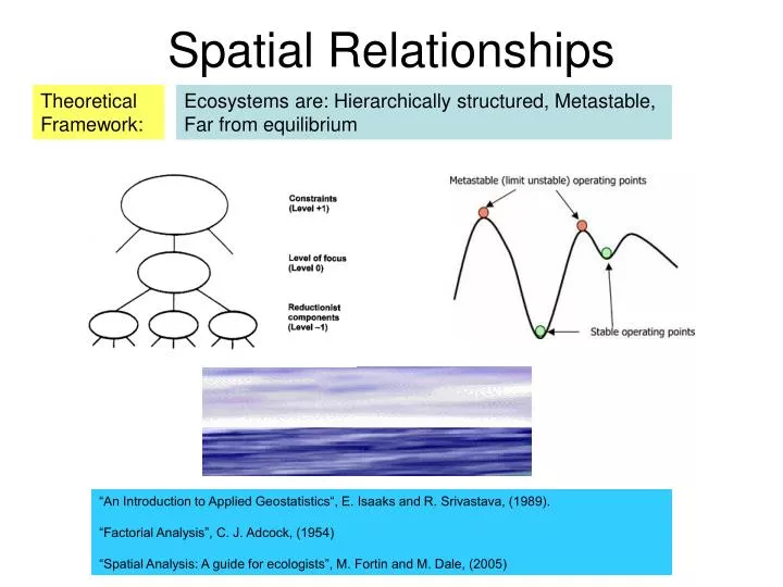
Spatial Relationships. Theoretical Framework:. Ecosystems are: Hierarchically structured, Metastable, Far from equilibrium. “An Introduction to Applied Geostatistics“, E. Isaaks and R. Srivastava, (1989). “Factorial Analysis”, C. J. Adcock, (1954)

E N D
Spatial Relationships Theoretical Framework: Ecosystems are: Hierarchically structured, Metastable, Far from equilibrium “An Introduction to Applied Geostatistics“, E. Isaaks and R. Srivastava, (1989). “Factorial Analysis”, C. J. Adcock, (1954) “Spatial Analysis: A guide for ecologists”, M. Fortin and M. Dale, (2005)
Variation Scale Distance Basic paradigm: Ecosystem processes (change) are constrained and controlled by the pattern of hierarchical scales “Things” closer together (in both space and time) are more alike then things far apart – “Tobler’s Law”(1970, Economic Geography) “Everything is related to everything, but near things are more related then distant things” Ecological “scale” is the space and time “distance” apart (lag) at which significant variation is NO LONGER correlated with “distance”
Applied Geostatistics Spatial Structure Regionalized Variable Spatial Autocorrelation Moran I (1950) GEARY C (1954) Semivariance Stationarity Anistotropy
Applied Geostatistics Notes on Introduction to Spatial Autocorrelation Geostatistical methods were developed for interpreting data that varies continuously over a predefined, fixed spatial region. The study of geostatistics assumes that at least some of the spatial variation observed for natural phenomena can be modeled by random processes with spatial autocorrelation. Geostatistics is based on the theory of regionalized variables, variabledistributed in space (or time). Geostatiscal theory supports that any measurement of regionalozed variables can be viewed as a realization of a random function (or random process, or random field, or stochastic process)
Spatial Structure Geostatistical techniques are designed to evaluate the spatial structure of a variable, or the relationship between a value measured at a point in one place, versus a value from another point measured a certain distance away. Describing spatial structure is useful for: • Indicating intensity of pattern and the scale at which that pattern is exposed • Interpolating to predict values at unmeasured points across the domain (e.g. kriging) • Assessing independence of variables before applying parametric tests of significance
A “structural” coarse scale forcing or trend A random” Local spatial dependency error variance (considered normally distributed) Regionalized Variable Regionalized Variables take on values according to spatial location. Given a variable z, measured at a location i, the variability in z can be broken down into three components: Usually removed by detrending Where: What we are interested in Coarse scale forcing or trends can be removed by fitting a surface to the trend using regression and then working with regression residuals
Z3 + Z2 + Z1 Zn + + Zi + Z4 + Z(x+h) Variables are spatially correlated, Therefore: Z(x+h) can be estimated from Z(x) by using a regression model. ** This assumption holds true with a recognized increased in error, from other lest square models. Z(x) Regionalized Variable Zi Function Z in domain D = a set of space dependent values Histogram of samples zi Cov(Z(x),Z(x+h))
Correlation: A Statement of the extent to which two data sets agree. Correlation Coefficient: Determined by the extent to which the two regressions lines depart from the horizontal and vertical. Two distributions One distribution θ2 ) a a ) θ1 ) θ b b As θ decreases, a/b goes to 0 deviates data x y x·y x2 y2 X 1 3 2 1 : : µ Y 3 2 5 3 : : µ If you were to calculate correlation by hand …. You would produce these Terms. Deviations Sum of squares Product of Deviations
CorrelationCoefficient = Spatial auto-correlation Briggs UT-Dallas GISC 6382 Spring 2007
:= Degree of correlation to self Autocorrelation: Spatial Autocorrelation: := The relationship is a function of distance Spatial Structure which is: Exogenous (induced) … induced external spatial dependence Endogenous (inherent) … inherent spatial autocorrelation Spatial Dependence: Compare values at given distance apart -- LAGS Point – Point Autocorrelation A - B Positive A - C None A - D Negative A BCD Anisotropic := varies in intensity and range with orientation Isotropic := varies similarly in all directions Direction of Autocorrelation: Spatial Structure
Spatial Pattern is an outcome of the synthesis of dynamic processes operating at various spatial and temporal scales Given: Therefore: Structure at any given time is but one realization of several potential outcomes Assuming: All processes are Stationary (homogeneous) Properties are independent of absolute location and direction in space Where: That is: Observations are independent which := they are homoscedastic and form a known distribution Therefore: Stationarity is a property of the process NOT the data allowing spatial inferences And: Furthermore: Stationarity is scale dependent Inference (spatial statistics) apply over regions of assumed stationarity Thus: Spatial Structure
J I H B G C F D A E Space Topological v’s Euclidean First Order Neighbors Topology Binary Connectivity Matrix Distance Class Connectivity Matrix A B C D E F G H I J A B C D E F G H I J A B C D E F G H I J A B C D E F G H I J 1= connected, 0=not connected
Spatial Autocorrelation A variable is thought to be autocorrelated if it is possible to predict its value at a given location, by knowing its value at other nearby locations. Positive autocorrelation: Negative autocorrelation: No autocorrelation: • Autocorrelation is evaluated using structure functions that assess the spatial structure or dependency of the variable. • Two of these functions are autocorrelation and semivariance which are graphed as a correlogram and semivariogram, respectively. • Both functions plot the spatial dependence of the variable against the spatial separation or lag distance.
A B C D E F G H I J K L Space Connectivity Matrix Euclidean Distance Matrix A B C D …. J A B C D …. J A 0.0 B 2.00 0.00 C 1.41 3.16 0.00 : : J A 0 B 0 0 C 1 0 0 : : J Euclidean Distance Matrix Weighted Matrix A B C D …. J A B C D …. J A 0 B 2 0 C 1 3 0 : : J A 0 B 0 0 C 0.7 0 0 D 0.7 0.7 0 : J
Moran I (1950) • A cross-product statistic that is used to describe autocorrelation • Compares value of a variable at one location with values at all other locations Where: n is the number of pairsZi is the deviation from the mean for value at location i (i.e., Zi= xi – x for variable x) Zj is the deviation from the mean for value at location j (i.e., Zj= xj – x for variable x) wijis an indicator function or weight at distance d (e.g. wij= 1, if j is in distance class d from point i, otherwise = 0) Wij is the sum of all weights (number of pairs in distance class) The numerator is a covariance (cross-product) term; the denominator is a variance term. Values range from [-1, 1] Value = 1 : Perfect positive correlation Value = -1: Perfect negative correlation
Moran I (1950) Again; where for variable x: n is the number of pairswij(d) is the distance class connectivity matrix (e.g. wij= 1, if j is in distance class d from point i, otherwise = 0) W(d) is the sum of all weights (number of pairs in distance class)
GEARY C (1954) • A squared difference statistic for assessing spatial autocorrelation • Considers differences in values between pairs of observations, rather than the covariation between the pairs (Moran I) The numerator in this equation is a defference term that gets squared. The Geary C statistic is more sensitive to extreme values & clustering than the Moran I, and behaves like a distance measure: Values range from [0,3] Value = 0 : Positive autocorrelation Value = 1 : No autocorrelation Value > 1 : Negative autocorrelation
Ripley’s K (1976) The L (d) transformations Determines if features are clustered at multiple different distance. Sensitive to study area boundary. Conceptualized as “number of points” within a set of radius sets. If events follow complete spatial randomness, the number of points in a circle follows a Poisson distribution (mean less then 1) and defines the “expected”. Where: A = area N = nuber of points D = distance K(i,j) = the weight, which is 1 when |i-j| < d, 0 when |i-j| > d
General G Effectively Distinguishes between “hot and cold” spots. G is relatively large if high values cluster, low if low values cluster. Numerator are “within” a distance bound (d), expressed relative to the entire study area. Where: d = distance class Wij = weight matrix, which is 1 when |i-j| < d, 0 when |i-j| > d
Semivariance The geostatistical measure that describes the rate of change of the regionalized variable is known as the semivariance. Semivariance is used for descriptive analysis where the spatial structure of the data is investigated using the semivariogram and for predictive applications where the semivariogram is fitted to a theoretical model, parameterized, and used to predict the regionalized variable at other non-measured points (kriging). Where : j is a point at distance d from i ndis the number of points in that distance class (i.e., the sum of the weights wij for that distance class) wij is an indicator function set to 1 if the pair of points is within the distance class.
A semivariogram is a plot of the structure function that, like autocorrelation, describes the relationship between measurements taken some distance apart. Semivariograms define the range or distance over which spatial dependence exists. • The nugget is the semivariance at a distance 0.0, (the y –intercept) • The sill is the value at which the semivariogram levels off (its asymptotic value) • The range is the distance at which the semivariogram levels off (the spatial extent of structure in the data)
Stationarity • Autocorrelation assumes stationarity, meaning that the spatial • structure of the variable is consistent over the entire domain of the dataset. • The stationarity of interest is second-order (weak) stationarity, requiring that: • the mean is constant over the region • variance is constant and finite; and • covariance depends only on between-sample spacing • In many cases this is not true because of larger trends in the data • In these cases, the data are often detrended before analysis. • One way to detrend data is to fit a regression to the trend, and use only the residuals for autocorrelation analysis
Anistotropy Autocorrelation also assumes isotropy, meaning that the spatial structure of the variable is consistent in all directions. Often this is not the case, and the variable exhibits anisotropy, meaning that there is a direction-dependent trend in the data. If a variable exhibits different ranges in different directions, then there is a geometric anisotropy. For example, in a dune deposit, larger range in the wind direction compared to the range perpendicular to the wind direction.
For predictions, the empirical semivariogram is converted to a theoretic one by fitting a statistical model (curve) to describe its range, sill, & nugget. There are four common models used to fit semivariograms: Assumes no sill or range Linear: Exponential: Spherical: Where: c0 = nugget b = regression slope a = range c0+ c = sill Gaussian:
Variogram Modeling Suggestions • Check for enough number of pairs at each lag distance (from 30 to 50). • Removal of outliers • Truncate at half the maximum lag distance to ensure enough pairs • Use a larger lag tolerance to get more pairs and a smoother variogram • Start with an omnidirectional variogram before trying directional variograms • Use other variogram measures to take into account lag means and variances (e.g., inverted covariance, correlogram, or relative variograms) • Use transforms of the data for skewed distributions (e.g. logarithmic transforms). • Use the mean absolute difference or median absolute difference to derive the range