Download
1 / 49
490 likes | 498 Views
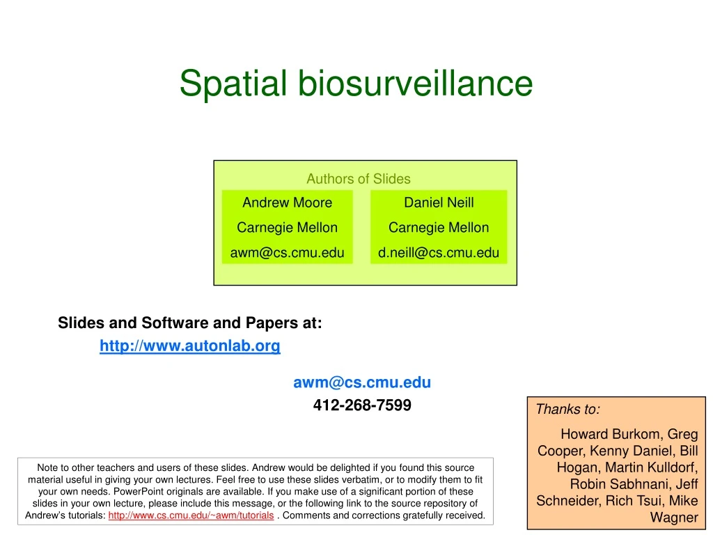
Authors of Slides. Andrew Moore Carnegie Mellon awm@cs.cmu.edu. Daniel Neill Carnegie Mellon d.neill@cs.cmu.edu. Spatial biosurveillance. Slides and Software and Papers at: http://www.autonlab.org. awm@cs.cmu.edu 412-268-7599. Thanks to:

E N D
Authors of Slides Andrew Moore Carnegie Mellon awm@cs.cmu.edu Daniel Neill Carnegie Mellon d.neill@cs.cmu.edu Spatial biosurveillance Slides and Software and Papers at: http://www.autonlab.org awm@cs.cmu.edu 412-268-7599 Thanks to: Howard Burkom, Greg Cooper, Kenny Daniel, Bill Hogan, Martin Kulldorf, Robin Sabhnani, Jeff Schneider, Rich Tsui, Mike Wagner Note to other teachers and users of these slides. Andrew would be delighted if you found this source material useful in giving your own lectures. Feel free to use these slides verbatim, or to modify them to fit your own needs. PowerPoint originals are available. If you make use of a significant portion of these slides in your own lecture, please include this message, or the following link to the source repository of Andrew’s tutorials: http://www.cs.cmu.edu/~awm/tutorials . Comments and corrections gratefully received.
Sverdlovsk • During April and May 1979, there were 77 Confirmed cases of inhalational anthrax
Goals of spatial cluster detection • To identify the locations, shapes, and sizes of potentially anomalous spatial regions. • To determine whether each of these potential clusters is more likely to be a “true” cluster or a chance occurrence. • In other words, is anything unexpected going on, and if so, where?
Disease surveillance Given: count for each zip code (e.g. number of Emergency Dept. visits, or over-the-counter drug sales, of a specific type) Do any regions have sufficiently high counts to be indicative of an emerging disease epidemic in that area? How many cases do we expect to see in each area? Are there any regions with significantly more cases than expected?
A simple approach • For each zip code: • Infer how many cases we expect to see, either from given denominator data (e.g. census population) or from historical data (e.g. time series of previous counts). • Perform a separate statistical significance test on that zip code, obtaining its p-value. • Report all zip codes that are significant at some level a. What are the potential problems?
A simple approach • For each zip code: • Infer how many cases we expect to see, either from given denominator data (e.g. census population) or from historical data (e.g. time series of previous counts). • Perform a separate statistical significance test on that zip code, obtaining its p-value. • Report all zip codes that are significant at some level a. One abnormal zip code might not be interesting… But a cluster of abnormal zip codes would be! What are the potential problems?
A simple approach Multiple hypothesis testing • For each zip code: • Infer how many cases we expect to see, either from given denominator data (e.g. census population) or from historical data (e.g. time series of previous counts). • Perform a separate statistical significance test on that zip code, obtaining its p-value. • Report all zip codes that are significant at some level a. Thousands of locations to test… 5% chance of false positive for each… Almost certain to get large numbers of false alarms! How do we bound the overall probability of getting any false alarms? What are the potential problems?
One Step of Spatial Scan Entire area being scanned
One Step of Spatial Scan Entire area being scanned Current region being considered
One Step of Spatial Scan Entire area being scanned Current region being considered I have a population of 5300 of whom 53 are sick (1%) Everywhere else has a population of 2,200,000 of whom 20,000 are sick (0.9%)
One Step of Spatial Scan Entire area being scanned Current region being considered I have a population of 5300 of whom 53 are sick (1%) So... is that a big deal? Evaluated with Score function. Everywhere else has a population of 2,200,000 of whom 20,000 are sick (0.9%)
Scoring functions • Define models: • of the null hypothesis H0: no attacks. • of the alternative hypotheses H1(S): attack in region S.
Scoring functions • Define models: • of the null hypothesis H0: no attacks. • of the alternative hypotheses H1(S): attack in region S. • Derive a score functionScore(S) = Score(C, B). • Likelihood ratio: • To find the most significant region:
Scoring functions C = Count in region B = Baseline (e.g. Population at risk) • Define models: • of the null hypothesis H0: no attacks. • of the alternative hypotheses H1(S): attack in region S. • Derive a score functionScore(S) = Score(C, B). • Likelihood ratio: • To find the most significant region:
Scoring functions Example: Kulldorf’s score Assumption: ci ~ Poisson(qbi) H0: q = qall everywhere H1: q = qin inside region, q = qout outside region • Define models: • of the null hypothesis H0: no attacks. • of the alternative hypotheses H1(S): attack in region S. • Derive a score functionScore(S) = Score(C, B). • Likelihood ratio: • To find the most significant region:
Scoring functions Example: Kulldorf’s score Assumption: ci ~ Poisson(qbi) H0: q = qall everywhere H1: q = qin inside region, q = qout outside region • Define models: • of the null hypothesis H0: no attacks. • of the alternative hypotheses H1(S): attack in region S. • Derive a score functionScore(S) = Score(C, B). • Likelihood ratio: • To find the most significant region: (Individually Most Powerful statistic for detecting significant increases) (but still…just an example)
The generalized spatial scan • Obtain data for a set of spatial locations si. • Choose a set of spatial regions S to search. • Choose models of the data under null hypothesis H0 (no clusters) and alternative hypotheses H1(S) (cluster in region S). • Derive a score function F(S) based on H1(S) and H0. • Find the most anomalous regions (i.e. those regions S with highest F(S)). • Determine whether each of these potential clusters is actually an anomalous cluster.
1. Obtain data for a set of spatial locations si. • For each spatial location si, we are given a count ci and a baseline bi. • For example: ci = # of respiratory disease cases, bi = at-risk population. • Goal: to find regions where the counts are higher than expected, given the baselines. ci = 20, bi = 5000 Population-based method: Expectation-based method: Baselines represent population, whether given (e.g. census) or inferred (e.g. from sales); can be adjusted for age, risk factors, seasonality, etc. Baselines represent expected counts, inferred from the time series of previous counts, accounting for day-of-week and seasonality effects. Under null hypothesis, we expect counts to be proportional to baselines. Under null hypothesis, we expect counts to be equal to baselines. Compare disease rate (count / pop) inside and outside region. Compare region’s actual count to its expected count.
1. Obtain data for a set of spatial locations si. • For each spatial location si, we are given a count ci and a baseline bi. • For example: ci = # of respiratory disease cases, bi = at-risk population. • Goal: to find regions where the counts are higher than expected, given the baselines. ci = 20, bi = 5000 Discussion question: When is it preferable to use each method? Population-based method: Expectation-based method: Baselines represent population, whether given (e.g. census) or inferred (e.g. from sales); can be adjusted for age, risk factors, seasonality, etc. Baselines represent expected counts, inferred from the time series of previous counts, accounting for day-of-week and seasonality effects. Under null hypothesis, we expect counts to be proportional to baselines. Under null hypothesis, we expect counts to be equal to baselines. Compare disease rate (count / pop) inside and outside region. Compare region’s actual count to its expected count.
2. Choose a set of spatial regions S to search. • Some practical considerations: • Set of regions should cover entire search space. • Adjacent regions should partially overlap. • Choose a set of regions that corresponds well with the size/shape of the clusters we want to detect. • Typically, we consider some fixed shape (e.g. circle, rectangle) and allow its location and dimensions to vary. Don’t search too few regions: Don’t search too many regions: Reduced power to detect clusters outside the search space. Overall power to detect any given subset of regions reduced because of multiple hypothesis testing. Computational infeasibility!
2. Choose a set of spatial regions S to search. • Our typical approach for disease surveillance: • map spatial locations to grid • search over the set of all gridded rectangular regions. • Allows us to detect both compact and elongated clusters (important because of wind- or water-borne pathogens). • Computationally efficient • can evaluate any rectangular region in constant time • can use fast spatial scan algorithm
2. Choose a set of spatial regions S to search. • Our typical approach for disease surveillance: • map spatial locations to grid • search over the set of all gridded rectangular regions. • Allows us to detect both compact and elongated clusters (important because of wind- or water-borne pathogens). • Computationally efficient • can evaluate any rectangular region in constant time • can use fast spatial scan algorithm Can also search over non-axis-aligned rectangles by examining multiple rotations of the data
3-4. Choose models of the data under H0 and H1(S), and derive a score function F(S). • Most difficult steps: must choose models which are efficiently computable and relevant.
3-4. Choose models of the data under H0 and H1(S), and derive a score function F(S). • Most difficult steps: must choose models which are efficiently computable and relevant. F(S) must be computable as function of some additive sufficient statistics of region S, e.g. total count C(S) and total baseline B(S).
3-4. Choose models of the data under H0 and H1(S), and derive a score function F(S). • Most difficult steps: must choose models which are efficiently computable and relevant. tradeoff! F(S) must be computable as function of some additive sufficient statistics of region S, e.g. total count C(S) and total baseline B(S). Any simplifying assumptions should not greatly affect our ability to distinguish between clusters and non-clusters.
3-4. Choose models of the data under H0 and H1(S), and derive a score function F(S). • Most difficult steps: must choose models which are efficiently computable and relevant. tradeoff! F(S) must be computable as function of some additive sufficient statistics of region S, e.g. total count C(S) and total baseline B(S). Any simplifying assumptions should not greatly affect our ability to distinguish between clusters and non-clusters. Iterative design process Test detection power Remove effect (preprocessing)? Y Calibrate High power? Basic model Done Filter out regions (postprocessing)? N Add complexity to model? Find unmodeled effect harming performance
3-4. Choose models of the data under H0 and H1(S), and derive a score function F(S). • Most difficult steps: must choose models which are efficiently computable and relevant. tradeoff! Discussion question: What effects should be treated with each technique? F(S) must be computable as function of some additive sufficient statistics of region S, e.g. total count C(S) and total baseline B(S). Any simplifying assumptions should not greatly affect our ability to distinguish between clusters and non-clusters. Iterative design process Test detection power Remove effect (preprocessing)? Y Calibrate High power? Basic model Done Filter out regions (postprocessing)? N Add complexity to model? Find unmodeled effect harming performance
Computing the score function Method 1 (Frequentist, hypothesis testing approach): Use likelihood ratio Prior probability of region S Method 2 (Bayesian approach): Use posterior probability What to do when each hypothesis has a parameter space Q? Method A (Maximum likelihood approach) Method B (Marginal likelihood approach)
Computing the score function Method 1 (Frequentist, hypothesis testing approach): Use likelihood ratio Most common (frequentist) approach: use likelihood ratio statistic, with maximum likelihood estimates of any free parameters, and compute statistical significance by randomization. Method A (Maximum likelihood approach)
5. Find the most anomalous regions, i.e. those regions S with highest F(S). • Naïve approach: compute F(S) for each spatial region S. • Better approach: apply fancy algorithms (e.g. Kulldorf’s SatScan or the fast spatial scan algorithm (Neill and Moore, KDD 2004). Problem: millions of regions to search!
5. Find the most anomalous regions, i.e. those regions S with highest F(S). • Naïve approach: compute F(S) for each spatial region S. • Better approach: apply fancy algorithms (e.g. Kulldorf’s SatScan or the fast spatial scan algorithm (Neill and Moore, KDD 2004). Problem: millions of regions to search! Start by examining large rectangular regions S. If we can show that none of the smaller rectangles contained in S can have high scores, we do not need to individually search each of these subregions. • Using a multiresolution data structure (overlap-kd tree) enables us to efficiently move between searching at coarse and fine resolutions.
5. Find the most anomalous regions, i.e. those regions S with highest F(S). Result: 20-2000x speedups vs. naïve approach, without any loss of accuracy • Naïve approach: compute F(S) for each spatial region S. • Better approach: apply fancy algorithms (e.g. Kulldorf’s SatScan or the fast spatial scan algorithm (Neill and Moore, KDD 2004). Problem: millions of regions to search! Start by examining large rectangular regions S. If we can show that none of the smaller rectangles contained in S can have high scores, we do not need to individually search each of these subregions. • Using a multiresolution data structure (overlap-kd tree) enables us to efficiently move between searching at coarse and fine resolutions.
6. Determine whether each of these potential clusters is actually an anomalous cluster. • Frequentist approach: calculate statistical significance of each region by randomization testing. D(S) = 21.2 D(S) = 15.1 D(S) = 18.5 Original grid G
6. Determine whether each of these potential clusters is actually an anomalous cluster. • Frequentist approach: calculate statistical significance of each region by randomization testing. … D(S) = 21.2 D*(G1) = 16.7 D*(G999) = 4.2 D(S) = 15.1 1. Create R = 999 replica grids by sampling under H0, using max-likelihood estimates of any free params. D(S) = 18.5 Original grid G
6. Determine whether each of these potential clusters is actually an anomalous cluster. • Frequentist approach: calculate statistical significance of each region by randomization testing. … D(S) = 21.2 D*(G1) = 16.7 D*(G999) = 4.2 D(S) = 15.1 1. Create R = 999 replica grids by sampling under H0, using max-likelihood estimates of any free params. D(S) = 18.5 Original grid G 2. Find maximum region score D* for each replica.
6. Determine whether each of these potential clusters is actually an anomalous cluster. • Frequentist approach: calculate statistical significance of each region by randomization testing. … D(S) = 21.2 D*(G1) = 16.7 D*(G999) = 4.2 D(S) = 15.1 1. Create R = 999 replica grids by sampling under H0, using max-likelihood estimates of any free params. D(S) = 18.5 Original grid G 2. Find maximum region score D* for each replica. 3. For each potential cluster S, count Rbeat = number of replica grids G’ with D*(G’) higher than D(S). 4. p-value of region S = (Rbeat+1)/(R+1). 5. All regions with p-value < a are significant at level a.
6. Determine whether each of these potential clusters is actually an anomalous cluster. • Bayesian approach: calculate posterior probability of each potential cluster. 1. Score of region S = Pr(Data | H1(S)) Pr(H1(S)) 2. Total probability of the data: Pr(Data) = Pr(Data | H0) Pr(H0) + ∑S Pr(Data | H1(S)) Pr(H1(S)) 3. Posterior probability of region S: Pr(H1(S) | Data) = Pr(Data | H1(S)) Pr(H1(S)) / Pr(Data). 4. Report all clusters with posterior probability > some threshold, or “sound the alarm” if total posterior probability of all clusters sufficiently high. Original grid G No randomization testing necessary… about 1000x faster than naïve frequentist approach!
Making the spatial scan fast 256 x 256 grid = 1 billion regions! Naïve frequentist scan 1000 replicas x 12 hrs / replica = 500 days! Fast frequentist scan Naïve Bayesian scan 1000 replicas x 36 sec / replica = 10 hrs 12 hrs (to search original grid) Fast Bayesian scan
Why the Scan Statistic speed obsession? • Traditional Scan Statistics very expensive, especially with Randomization tests • Going national • A few hours could actually matter!
Summary of results • The fast spatial scan results in huge speedups (as compared to exhaustive search), making fast real-time detection of clusters feasible. • No loss of accuracy: fast spatial scan finds the exact same regions and p-values as exhaustive search. OTC data from National Retail Data Monitor ED data
Performance comparison • On ED dataset (600,000 records), 1000 replicas • For SaTScan: M=17,000 distinct spatial locations • For Exhaustive/fast: 256 x 256 grid
Performance comparison • Algorithms: Neill and Moore, NIPS 2003, KDD 2004 • Deployment: Neill, Moore, Tsui and Wagner, Morbidity and Mortality Weekly Report, Nov. ‘04 • On ED dataset (600,000 records), 1000 replicas • For SaTScan: M=17,000 distinct spatial locations • For Exhaustive/fast: 256 x 256 grid
d-dimensional partitioning • Parent region S is divided into 2d overlapping children: an “upper child” and a “lower child” in each dimension. • Then for any rectangular subregion S’ of S, exactly one of the following is true: • S’ is contained entirely in (at least) one of the children S1… S2d. • S’ contains the center region SC, which is common to all the children. • Starting with the entire grid G and repeating this partitioning recursively, we obtain the overlap-kd tree structure. S1 S5 S2 S3 S S4 SC S6 • Algorithm: Neill, Moore and Mitchell NIPS 2004
Limitations of the algorithm • Data must be aggregated to a grid. • Not appropriate for very high-dimensional data. • Assumes that we are interested in finding (rotated) rectangular regions. • Less useful for special cases (e.g. square regions, small regions only). • Slower for finding multiple regions.
Related work • non-specific clustering: evaluates general tendency of data to cluster • focused clustering: evaluates risk w.r.t. a given spatial location (e.g. potential hazard) • disease mapping: models spatial variation in risk by applying spatial smoothing. • spatial scan statistics (and related techniques).