Download
1 / 23
230 likes | 362 Views
Issues and procedures regarding the simulation of current radiance observations. Ronald M. Errico UMBC/GEST NASA/GMAO. Outline. Lessons from previous OSSEs What are the important issues? Simulation of cloud cleared locations

E N D
Issues and procedures regarding the simulation of current radiance observations Ronald M. Errico UMBC/GEST NASA/GMAO
Outline • Lessons from previous OSSEs • What are the important issues? • Simulation of cloud cleared locations • Simulation of errors remaining after QC
(J/Kg) (J/Kg) Impacts of various observing systems Totals GEOS-5 July 2005 NH observations Observation Count (millions) …all observing systems provide total monthly benefit SH observations Observation Count (millions) From R. Gelaro & Y. Zhu
OSSE produced by Michiko et al. using T213L31 ECMWF T170 assimilation Includes radiances
OSSE produced by Michiko et al. using T213L31 ECMWF T170 assimilation No radiances
Decide what characteristics of observations and their errors are critical to duplicate (and by how close an approximation) • The above decision depends on: • How well the OSSE validation test criteria are to be satisfied • How much development time is to be invested My suggestion: Let’s not aim for perfection for the new control simulations (i.e., the ones using current operational observation data types), but let’s strive to do significantly better than for previous OSSEs
Issues: • Simulate realistic distributions of locations of accepted observations • Simulate error-free, cloud-free radiances • Simulate realistic distributions of instrument plus • representativeness error for observations
Simulate locations of QC accepted observation • Objectives: • 1. Accepted observation count similar to that of real data • 2. Geographical distribution similar to that of real data • (in what subjective or measurable senses?) • Considerations • Cloud screening or clearing • Other causes for QC rejection ? • Specification of Obs values to cause QC rejection
Accepted Observation Locations NOAA 17 HIRS Ch. 5 7/23/05 NOAA 17 HIRS Ch. 5 7/18/05 From Y. Zhu
Distribution of Accepted AIRS Obervations over 12-hour Period From Y. Zhu
Validation of simulated locations Ideally, the simulation of locations is validated, if global maps of simulated observation locations for individual observing periods are indistinguishable from random maps of real observation locations for equivalent periods.
Cloud Related Nature Run Fields 2-D: Low cloud fractional coverage Medium cloud fractional coverage High cloud fractional coverage Total cloud cover Convective precipitation Stratiform precipitation 3-D Cloud liquid water content Cloud ice water content Cloud Cover
Our modest goal need not be to simulate the radiances from cloudy regions, but more simply to get the geographical distribution and selected innovation statistics “realistic.” This is simpler because most details regarding the clouds are irrelevant.
Algorithm for determining cloud-cleared observation locations For each grid box where a satellite observation is given, use the cloud fraction to specify probability that it is a clear spot. Then use random number to specify whether pixel is clear. Use a functional relationship between probability and cloud fraction that we can tune to get a reasonable distribution.
Strawman procedure for simulating observations • For each observation location …… • Bilinearly interpolate cloud fractions from NR grid to location • Compute P(f, tuning parameter) • Select random number x from uniform distribution (0,1) • If x>P then consider cloud free for this height of cloud, • otherwise cloud covered point • If cloud free, then bilinearly interpolate q,T to location and • compute radiances for these unaffected channels • If cloudy region, set radiance to very small value such that • QC will detect and discard. • Repeat this process with various tuning parameters for P until • the observation count and distribution look reasonable. Then • use this parameter for all further experiments.
Simulation of error-free radiances Information required from nature run: T q Ps Ts Surface information that affects emmisivity
Instrument Plus Representativeness Error • Since we have no real instrument, its errors must be entirely simulated. • If different radiative transfer models (more generally called “forward • models” or “observation operators”) are used for simulation and • assimilation, then a portion of representativness error has already been added. • The assimilation uses an interpolation algorithm (another form of forward • model) for interpolating from fields defined at analysis grid points to values • specified at observation locations. Similar models are also applied to the nature • run for simulated observation locations. Since the assimilation and N.R. grids • differ in resolution, there is another source for differing relationships between • grid point values. For these reasons, another portion of representativness error • has already been added when the simulated observations were created.
Error statistics to consider Note: Real errors are likely functions of geography, local flow, season, viewing angle, etc., and are mutually correlated. 1. Biases: My recommendation is simply set to 0 2. Variances: My recommendation is simply set to constant that is a function of channel only. 3. Correlations: My recommendation is to assume no correlation. 4. Distribution function: My recommendation is to use a Gaussian (since these are applied to only those simulated observations that are intended to pass QC). It is difficult to produce more realistic statistics without better guidance regarding what those statistics are. It may also be unnecessary.
Strawman procedure for simulating instrument plus representativeness errors • Obtain an estimate of the statistics of representativeness error • due to using 2 different RT models (biases and variances) • Obtain an estimate of the statistics of representativeness error • due to differing grid resolutions and bilinear interpolation • Generate errors to be added to each observation by drawing • random numbers from a N(R’,0) distribution. Ignore biases • since any large bias will be removed by the assimilation anyway. • Use R’<R, R being the error value specified in the DAS. • Run the assimilation for a short time and note the variance of • the innovations. Re-adjust R’ so that this variance better matches • the corresponding variance computed for the real assimilation. • After 1 or 2 iterations of this, use the final R’ in any further experiments. Note: 1 and 2 are not strictly necessary for this purpose since they only help in defining an initial iterate for R’. For interpreting results, however, they should be very helpful. Otherwise a starting value for R’ can be, e.g., R’=2R/3.