Download
1 / 26
260 likes | 427 Views
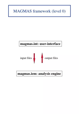
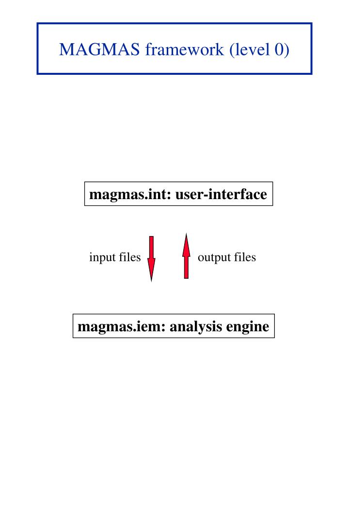
MAGMAS framework (level 0). magmas.int: user-interface. input files. output files. magmas.iem: analysis engine. magmas.int: user interface (level 1). print. view. file. matlab. magmas.int. calculate.IEM. patch_and_ap- erture_designer. engine. edit_ optim_ param. edit_ phys_

E N D
MAGMAS framework (level 0) magmas.int: user-interface input files output files magmas.iem: analysis engine
magmas.int: user interface (level 1) print view file matlab magmas.int calculate.IEM patch_and_ap- erture_designer engine edit_ optim_ param edit_ phys_ param edit_ freq_ param edit_ exc_ param edit_ gen_ param edit_ num_ param draw
edit_patch edit_aperture edit_wall edit_probe rectangle open_draw_window edit_phys_param (level 2) edit_layer edit_subreg edit_shlay edit_connect edit_phys_param builds main edit window load_view3D edit_element edit_pa_ap_act edit_eltype specify curr. distribution edit_slot patch_and_ aperture_ designer general get dimensions get dimensions edit_draw_wall edit_wall_sideview patch drawing window draw meshing
read_draw_graph_szy passes data to matlab and draws read_draw_graph_f passes data to matlab and draws read_draw_graph_p passes data to matlab and draws view (level 2) load_view3D read_szy reads data from s,z,y.out file graph_y Y-parameters graph_z Z-parameters edit_graphs_szy - sets up plot window - gets plot parameters graph_s view S-parameters graph_f single port FF edit_graphs_fp - sets up plot window - gets plot parameters graph_p structure FF graph_i current and charge opt_plot opt. & param. plots
graph_i view (level 2) edit_graphs_i sets up current plot window actify read_display_curr imposes the loaded current on an active patch find_magc2 read_current_to matlab finds the engine sheet- current number (c2) read & display curr.
magmas.iem: analysis engine (level 1) input: read input exc.dta mesher: meshing MIDAS: layer structure PTLS: transmission lines ETed: element types trunc + FFWo + FF_PO3: finite layer structure sortSR + linkSR: subregion coupling DBD_GN: de-embedding WiWof + WiWoT + AY: element coupling LiLof + NW: element linking no optimisation completed ? yes calculation network parameters output: write output exc: excitations exc.dta
midas: layer structure (level 2) SPECTRAL: spectral GFs INVFT3D: inverse FT INVFT2D: inverse FT spatial3D: 3D spatial GFs spatial2D: 2D spatial GFs FarField: 3D spectral FF
spectral: spectral GFs (level 3) c = current sheet p = probe PARAM: parameters PPmodes: probe disc systems SING: singularities storeEW: expansion waves BFbpser: BP-series BFas: asymptotes COhh, COvh, COhv, COvv, COcp, COpc, COpp: coefficients for problematic behavior BFas2: numerical asymptotes BFB: basic spectral GFs BFsi: annihilating functions BFcchh, BFccvh, BFcchv, BFccvv, BFcp, BFpc, BFpp: spectral GFs
spatial3D: 3D spatial GFs (level 3) c = current sheet p = probe RFsi: annihilating functions for singularities RFashh, RFashvvh, RFcph, RFpch, RFpph: annihilating functions for asymptotes RFhh, RFhvvh, RFcp, RFpc, RFpp, RFpf: 3D spatial GFs
spatial2D: 2D spatial GFs (level 3) c = current sheet RFsi2D: annihilating functions for singularities RFcch2D: annihilating functions for asymptotes RFcc2D: 2D spatial GFs
PTLS: transmission line types (level 2) Muller: propagation constants characteristic impedances current profile
Muller: propagation constants(level 3) CC_FN: spatial points CC_FN: normalization factor CC_FN: initial values CC_FN: root calculation no convergence yes MOCUR: modal currents Zc: modal power
CC_FN: characteristic function (level 4) Midas_2d: Green’s functions ELMCOP: overall coupling STRPRD: solve electric currents MIXER: solve magnetic currents Normalize + calculate determinant
ELMCOP: overall coupling matrix (level 5) REACTN: calculates the coupling between each set of two basis functions REACTN … REACTN
REACTN: basis function coupling (level 6) DETGNF: select appropriate GFs INNPRO + GFXPOL: calculate coupling
ETed: element types (level 2) ETsu: subsectional active current sheet and wall reduction
ETsu: subsectional (level 3) [1] ChChs, ChChs_gal: Ch to Ch (self) ChChms, ChChms_gal, ChChmm: Ch to Ch (mutual) CvChm, CvChe: Ch to Cv CvCv: Cv to Cv Ch = horizontal current sheet Cv = vertical current sheet Cc = connecting current sheet PB = probe EW = exp. wave ChmCv, CheCv: Cv to Ch CcChm, CcChe: Ch to Cc CcCv: Cv to Cc CcCc: Cc to Cc CvCc: Cc to Cv ChmCc, CheCc: Cc to Ch
ETsu: subsectional (level 3) [2] PChs, PChm: Ch to P ChPs, ChPm: P to Ch PBPB: PB to PB Ch = horizontal current sheet Cv = vertical current sheet Cc = connecting current sheet PB = probe EW = exp. wave EWPs, EWAs: Ch to EW ChEWn, ChEWp: EW to Ch EWP: P to EW PEWp: EW to P
ETsu: subsectional (level 3) [3] EW to EW Ch to coaxial feed coaxial feed to Ch P to coaxial feed Ch = horizontal current sheet P = probe EW = exp. wave coaxial feed to P coaxial feed to EW EW to coaxial feed coaxial feed to coaxial feed
ETsu: subsectional (level 3) [4] elimination passive electric current sheets and probes FcPa: FF by active patches Ch = current sheet P = probe EW = exp. wave FF = far field FcPp: FF by passive patches FP: FF by probes FcA: FF by apertures FF: spherical system
finite layer structure (level 1) trunc: expansion wave diffraction (only called for 2D SIE) FF_Wo: outgoing wave →diffraction → far field (called for 2D SIE) FF_PO3: outgoing wave →diffraction → far field (called for 3D VPO)
trunc: 2D SIE Diffraction coefficients (level 2) DC = Diffraction Coefficient FORM_FM: basis functions dc_sie: FORM_FM: incident current df_cfg: description of edge for SIE calc_all: DC for each expansion wave
calc_all: 2D SIE DC for each expansion wave (level 3) IC = incident current CM = coupling matrix FORM_FN: recount of basis functions form_cur: modification of IC form_frg: current for region calc_yy: region CM dc_prh: IC right part invert: solution DIFR: 2D Far Field d_reflF: 2D reflected waves
calc_yy: coupling matrix (level 4) BF= basis functions c_ybs: annihilating functions for poles simpson2: IFT of calc_y, dc_pg2 (coupling matrices in spectral domain) frm_y: coupling matrix in spectral domain frm_w: spectral region parameters d_idl: BF integrals couple, couplez: layer spectral parameters y_xx, y_xz:spectralcoupling between 2 BF calc_ya: asymptote calc_ys: coupling matrix in free space
FF_PO3: outgoing wave far field coupling using 2D VPO (level 3) VC = volume currents LCS = local coordinate system df_eps: auxiliary region parameters dc_PO3, simp_PO3: integral over φ’ df_PO3: VC integral over r’ and z’ df_crnT: corners positions in LCS df_sZ: VC integral over z’
FFWo: outgoing wave far field coupling using 2D SIE (level 3) DC = diffraction coefficient DP = point of diffraction Ananke: modification of space wave DC df_pdc: input DC from file EE_Wout: outgoing wave > far field veronika: auxiliary points at the edge lisa: DP+ diffraction angles ATT: EW amplitude at DP pDTM: 3D DC from 2D DC