Download
1 / 22
220 likes | 310 Views
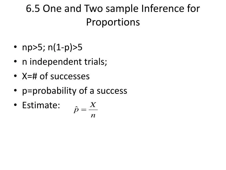
6.5 One and Two sample Inference for Proportions. np >5; n(1-p)>5 n independent trials; X=# of successes p=probability of a success Estimate:. Mean and variance of.

E N D
6.5 One and Two sample Inference for Proportions • np>5; n(1-p)>5 • n independent trials; • X=# of successes • p=probability of a success • Estimate:
Mean and variance of When n is large, approximate probabilities for can be found using the normal distribution with the same mean and standard deviation.
Sample Size • The sample size required to have a certain probability that our error (plus or minus part of the CI) is no more than size ∆ is
If you know p is somewhere … • If then maximum p(1-p)=0.3(1-0.3)=0.21 • If then maximum p(1-p)=0.4(1-0.4)=0.24
Estimate p(1-p) by substitute p with the value closest to 0.5 (0, 0.1), p=0.1 (0.3, 0.4), p=0.4 (0.6, 1.0), p=0.6
Example • A state highway dept wants to estimate what proportion of all trucks operating between two cities carry too heavy a load • 95% probability to assert that the error is no more than 0.04 • Sample size needed if • p between 0.10 to 0.25 • no idea what p is
Solution • ∆=0.04, p=0.25 Round up to get n=451 • ∆=0.04, p(1-p)=1/4 n=601
Tests of Hypotheses • Null H0: p=p0 • Possible Alternatives: HA: p<p0 HA: p>p0 HA: pp0
Test Statistics • Under H0, p=p0, and • Statistic: is approximately standard normal under H0 . Reject H0 if z is too far from 0 in either direction.
Example • H0: p=0.75 vs HA: p0.75 • =0.05 • n=300 • x=206 • Reject H0 if z<-1.96 or z>1.96
Observed z value • Conclusion: reject H0 since z<-1.96 • P(z<-2.5 or z>2.5)=0.0124<a reject H0.
Example • Toss a coin 100 times and you get 45 heads • Estimate p=probability of getting a head Is the coin balanced one? a=0.05 Solution: H0: p=0.50 vs HA: p0.50
Enough Evidence to Reject H0? • Critical value z0.025=1.96 • Reject H0 if z>1.96 or z<-1.96 • Conclusion: accept H0
Truth = surgical biopsy Cancer Present Cancer Absent Total Result Positive 140 80 220 FNA status Results Negative 10 910 920 150 990 1140 Total Another example • The following table is for a certain screening test
Test to see if the sensitivity of the screening test is less than 97%. • Hypothesis • Test statistic
What is the conclusion? • Check p-value when z=-2.6325, p-value = 0.004 • Conclusion: we can reject the null hypothesis at level 0.05.
Truth = surgical biopsy Cancer Present Cancer Absent Total Result Positive 14 8 22 FNA status Results Negative 1 91 92 114 15 99 Total One word of caution about sample size: • If we decrease the sample size by a factor of 10,
And if we try to use the z-test, P-value is greater than 0.05 for sure (p=0.2026). So we cannot reach the same conclusion. And this is wrong!
So for test concerning proportions We want np>5; n(1-p)>5