Download
1 / 43
540 likes | 1.04k Views
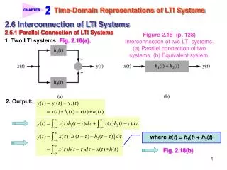
2. CHAPTER. Time-Domain Representations of LTI Systems. 2.6 Interconnection of LTI Systems. Figure 2.18 (p. 128) Interconnection of two LTI systems. (a) Parallel connection of two systems. (b) Equivalent system. 2.6.1 Parallel Connection of LTI Systems. 1. Two LTI systems: Fig. 2.18(a).

E N D
2 CHAPTER Time-Domain Representations of LTI Systems 2.6 Interconnection of LTI Systems Figure 2.18 (p. 128)Interconnection of two LTI systems. (a) Parallel connection of two systems. (b) Equivalent system. 2.6.1 Parallel Connection of LTI Systems 1. Two LTI systems: Fig. 2.18(a). 2. Output: where h(t) = h1(t) + h2(t) Fig. 2.18(b)
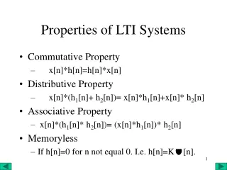
2 CHAPTER Time-Domain Representations of LTI Systems Distributive property for Continuous-time case: (2.15) Distributive property for Discrete-time case: (2.16) 2.6.2 Cascade Connection of LTI Systems 1. Two LTI systems: Fig. 2.19(a). Figure 2.19 (p. 128)Interconnection of two LTI systems. (a) Cascade connection of two systems. (b) Equivalent system. (c) Equivalent system: Interchange system order.
2 CHAPTER Time-Domain Representations of LTI Systems 2. The output is expressed in terms of z(t) as (2.17) (2.18) Since z(t) is the output of the first system, so it can be expressed as (2.19) Substituting Eq. (2.19) for z(t) into Eq. (2.18) gives Change of variable = (2.20) Define h(t) = h1(t) h2(t), then Fig. 2.19(b). (2.21) 3. Associative property for continuous-time case:
2 CHAPTER Time-Domain Representations of LTI Systems (2.22) 4. Commutative property: Write h(t) = h1(t) h2(t) as the integral Change of variable = t Fig. 2.19(c). (2.23) Interchanging the order of the LTI systems in the cascade without affecting the result: Commutative property for continuous-time case: (2.24) 5. Associative property for discrete-time case: (2.25) Commutative property for discrete-time case: (2.26)
2 CHAPTER Time-Domain Representations of LTI Systems Example 2.11Equivalent System to Four Interconnected Systems Consider the interconnection of four LTI systems, as depicted in Fig. 2.20. The impulse responses of the systems are and Find the impulse response h[n] of the overall system. Figure 2.20 (p. 131)Interconnection of systems for Example 2.11. <Sol.> 1. Parallel combination of h1[n] and h2[n]: h12[n] = h1[n] + h2[n] Fig. 2.21 (a).
2 CHAPTER Time-Domain Representations of LTI Systems Figure 2.21 (p. 131)(a) Reduction of parallel combination of LTI systems in upper branch of Fig. 2.20. (b) Reduction of cascade of systems in upper branch of Fig. 2.21(a). (c) Reduction of parallel combination of systems in Fig. 2.21(b) to obtain an equivalent system for Fig. 2.20.
2 CHAPTER Time-Domain Representations of LTI Systems 2. h12[n] is in series with h3[n]: h123[n] = h12[n] h3[n] h123[n] = (h1[n] + h2[n]) h3[n] Fig. 2.21 (b). 3. h123[n] is in parallel with h4[n]: h[n] = h123[n] h4[n] Fig. 2.21 (c). Thus, substitute the specified forms of h1[n] and h2[n] to obtain Convolving h12[n] with h3[n] gives Table 2.1 summarizes the interconnection properties presented in this section.
2 CHAPTER Time-Domain Representations of LTI Systems 2.7 Relation Between LTI System Properties and the Impulse Response 2.7.1 Memoryless LTI Systems 1. The output of a discrete-time LTI system: (2.27)
2 CHAPTER Time-Domain Representations of LTI Systems 2. To be memoryless, y[n] must depend only on x[n] and therefore cannot depend on x[n k] for k 0. A discrete-time LTI system is memoryless if and only if c is an arbitrary constant Continuous-time system: 1. Output: 2. A continuous-time LTI system is memoryless if and only if c is an arbitrary constant 2.7.2 Causal LTI Systems The output of a causal LTI system depends only on past or present values of the input. Discrete-time system: 1. Convolution sum:
2 CHAPTER Time-Domain Representations of LTI Systems 2. For a discrete-time causal LTI system, 3. Convolution sum in new form: Continuous-time system: 1. Convolution integral: 3. Convolution integral in new form: 2. For a continuous-time causal LTI system, 2.7.3 Stable LTI Systems A system is BIBO stable if the output is guaranteed to be bounded for every bounded input. Output: Discrete-time case: Input
2 CHAPTER Time-Domain Representations of LTI Systems 1. The magnitude of output: 2. Assume that the input is bounded, i.e., and it follows that (2.28) Hence, the output is bounded, or y[n] ≤ for all n, provided that the impulse response of the system is absolutely summable. 3. Condition for impulse response of a stable discrete-time LTI system:
2 CHAPTER Time-Domain Representations of LTI Systems Continuous-time case: Condition for impulse response of a stable continuous-time LTI system: Example 2.12Properties of the First-Order Recursive System The first-order system is described by the difference equation and has the impulse response Is this system causal, memoryless, and BIBO stable? <Sol.> 1. The system is causal, since h[n] = 0 for n < 0. 2. The system is not memoryless, since h[n] 0 for n > 0. 3. Stability: Checking whether the impulse response is absolutely summable?
2 CHAPTER Time-Domain Representations of LTI Systems if and only if < 1 ◆ Note: A system can be unstable even though the impulse response has a finite value. 1. Ideal integrator: (2.29) Input: x() = (), then the output is y(t) = h(t) = u(t). h(t) is not absolutely integrable Ideal integrator is not stable! 2. Ideal accumulator: Impulse response: h[n] = u[n] h[n] is not absolutely summable Ideal accumulator is not stable!
2 CHAPTER Time-Domain Representations of LTI Systems 2.7.4 Invertible Systems and Deconvolution A system is invertible if the input to the system can be recovered from the output except for a constant scale factor. 1. h(t) = impulse response of LTI system, 2. hinv(t) = impulse response of LTI inverse system Fig. 2.24. Figure 2.24 (p. 137)Cascade of LTI system with impulse response h(t) and inverse system with impulse response h-1(t). 3. The process of recovering x(t) from h(t) x(t) is termed deconvolution. 4. An inverse system performs deconvolution. Continuous-time case (2.30) 5. Discrete-time case: (2.31)
2 CHAPTER Time-Domain Representations of LTI Systems Example 2.13Multipath Communication Channels: Compensation by means of an Inverse System Consider designing a discrete-time inverse system to eliminate the distortion associated with multipath propagation in a data transmission problem. Assume that a discrete-time model for a two-path communication channel is Find a causal inverse system that recovers x[n] from y[n]. Check whether this inverse system is stable. <Sol.> 1. Impulse response: 2. The inverse system hinv[n] must satisfy h[n] hinv[n] = [n]. (2.32) • For n < 0, we must have hinv[n] = 0 in order to obtain a causal inverse • system
2 CHAPTER Time-Domain Representations of LTI Systems 2) For n = 0, [n] = 1, and eq. (2.32) implies that (2.33) 3. Since hinv[0] = 1, Eq. (2.33) implies that hinv[1] = a, hinv[2] = a2, hinv[3] = a3, and so on. The inverse system has the impulse response 4. To check for stability, we determine whether hinv[n] is absolutely summable, which will be the case if is finite. For a < 1, the system is stable. ★ Table 2.2 summarizes the relation between LTI system properties and impulse response characteristics.
2 CHAPTER Time-Domain Representations of LTI Systems 2.8 Step Response 1. The step response is defined as the output due to a unit step input signal. 2. Discrete-time LTI system: Let h[n] = impulse response and s[n] = step response. 3. Since u[n k] = 0 for k > n and u[n k] = 1 for k≤ n, we have
2 CHAPTER Time-Domain Representations of LTI Systems The step response is the running sum of the impulse response. Continuous-time LTI system: (2.34) The step response s(t) is the running integral of the impulse response h(t). ◆ Express the impulse response in terms of the step response as and Figure 2.12 (p. 119)RC circuit system with the voltage source x(t) as input and the voltage measured across the capacitor y(t), as output. Example 2.14RC Circuit: Step Response The impulse response of the RC circuit depicted in Fig. 2.12 is Find the step response of the circuit. <Sol.>
2 CHAPTER Time-Domain Representations of LTI Systems 1. Step response: Figure 2.25 (p. 140)RC circuit step response for RC = 1 s. Fig. 2.25
2 CHAPTER Time-Domain Representations of LTI Systems 2.9 Differential and Difference Equation Representations of LTI Systems 1. Linear constant-coefficient differential equation: Input = x(t), output = y(t) (2.35) 2. Linear constant-coefficient difference equation: Input = x[n], output = y[n] (2.36) The order of the differential or difference equation is (N, M), representing the number of energy storage devices in the system. Often, N M, and the order is described using only N. Ex. RLC circuit depicted in Fig. 2.26. 1. Input = voltage source x(t), output = loop current 2. KVL Eq.:
2 CHAPTER Time-Domain Representations of LTI Systems Figure 2.26 (p. 141)Example of an RLC circuit described by a differential equation. N = 2 Ex. Accelerator modeled in Section 1.10: N = 2 where y(t) = the position of the proof mass, x(t) = external acceleration.
2 CHAPTER Time-Domain Representations of LTI Systems Ex. Second-order difference equation: (2.37) N = 2 Difference equations are easily rearranged to obtain recursive formulas for computing the current output of the system from the input signal and the past outputs. Ex. Eq. (2.36) can be rewritten as Ex. Consider computing y[n] for n 0 from x[n] for the second-order difference equation (2.37). <Sol.> 1. Eq. (2.37) can be rewritten as (2.38) 2. Computing y[n] for n 0:
2 CHAPTER Time-Domain Representations of LTI Systems (2.39) (2.40) Initial conditions: y[ 1] and y[ 2]. ◆ The initial conditions for Nth-order difference equation are the N values ◆ The initial conditions for Nth-order differential equation are the N values
2 CHAPTER Time-Domain Representations of LTI Systems Example 2.15Recursive Evaluation of a Difference Equation Find the first two output values y[0] and y[1] for the system described by Eq. (2.38), assuming that the input is x[n] = (1/2)nu[n] and the initial conditions are y[ 1] = 1 and y[ 2] = 2. <Sol.> 1. Substitute the appropriate values into Eq. (2.39) to obtain 2. Substitute for y[0] in Eq. (2.40) to find Example 2.16Evaluation of a Difference Equation by means of a Computer A system is described y the difference equation Write a recursive formula that computes the present output from the past outputs and the current inputs. Use a computer to determine the step response
2 CHAPTER Time-Domain Representations of LTI Systems of the system, the system output when the input is zero and the initial conditions are y[ 1] = 1 and y[ 2] = 2, and the output in response to the sinusoidal inputs x1[n] = cos(n/10), x2[n] = cos(n/5), and x3[n] = cos(7n/10), assuming zero initial conditions. Last, find the output of the system if the input is the weekly closing price of Intel stock depicted in Fig. 2.27, assuming zero initial conditions. <Sol.> 1. Recursive formula for y[n]: 2. Step response: Fig. 2.28 (a). 3. Zero input response: Fig. 2.28 (b). 4. The outputs due to the sinusoidal inputs x1[n], x2[n], and x3[n]: Fig. 2.28 (c), (d), and (e). 5. Fig. 2.28(f) shows the system output for the Intel stock price unit. A comparison of peaks in Figs. 2.27 and 2.28 (f) Slightly delay!
2 CHAPTER Time-Domain Representations of LTI Systems Figure 2.27 (p. 144)Weekly closing price of Intel stock.
2 CHAPTER Time-Domain Representations of LTI Systems Fig. 2.28 (a).
2 CHAPTER Time-Domain Representations of LTI Systems Fig. 2.28 (b).
2 CHAPTER Time-Domain Representations of LTI Systems Fig. 2.28 (c). Fig. 2.28 (d).
2 CHAPTER Time-Domain Representations of LTI Systems Fig. 2.28 (e). Figure 2.28a (p. 145)Illustration of the solution to Example 2.16. (a) Step response of system. (b) Output due to nonzero initial conditions with zero input. (c) Output due to x1[n] = cos (1/10n). (d) Output due to x2[n] = cos (1/5n). (e) Output due to x3[n] = cos(7/10n).
2 CHAPTER Time-Domain Representations of LTI Systems Figure 2.28f (p. 146)Output associated with the weekly closing price of Intel stock.
2 CHAPTER Time-Domain Representations of LTI Systems 2.10 Solving Differential and Difference Equations Complete solution: y = y(h) + y(p) y(h) = homogeneous solution, y(p) = particular solution 2.10.1 The Homogeneous Solution Continuous-time case: 1. Homogeneous differential equation: 2. Homogeneous solution: Coefficients ci is determined by I.C. (2.41) 3. Characteristic eq.: (2.42) Discrete-time case: 1. Homogeneous differential equation: 2. Homogeneous solution: Coefficients ci is determined by I.C. (2.43) 3. Characteristic eq.: (2.44)
2 CHAPTER Time-Domain Representations of LTI Systems If a root rj is repeated p times in characteristic eqs., the corresponding solutions are Continuous-time case: Discrete-time case: Example 2.17RCCircuit: Homogeneous Solution The RC circuit depicted in Fig. 2.30 is described by the differential equation Determine the homogeneous solution of this equation. <Sol.> 1. Homogeneous Eq.: Figure 2.30 (p. 148)RC circuit. 2. Homo. Sol.: r1 = 1/RC 3. Characteristic eq.: 4. Homogeneous solution:
2 CHAPTER Time-Domain Representations of LTI Systems Example 2.18First-OrderRecursive System: Homogeneous Solution Find the homogeneous solution for the first-order recursive system described by the difference equation <Sol.> 1. Homogeneous Eq.: 2. Homo. Sol.: r1 = 3. Characteristic eq.: 4. Homogeneous solution: 2.10.2 The Particular Solution A particular solution is usually obtained by assuming an output of the same general form as the input. Table 2.3
2 CHAPTER Time-Domain Representations of LTI Systems Example 2.19First-OrderRecursive System (Continued): Particular Solution Find a particular solution for the first-order recursive system described by the difference equation if the input is x[n] = (1/2)n. <Sol.> 1. Particular solution form: 2. Substituting y(p)[n] and x[n] into the given difference Eq.:
2 CHAPTER Time-Domain Representations of LTI Systems Both sides of above eq. are multiplied by (1/2) n (2.45) 3. Particular solution: Figure 2.30 (p. 148)RC circuit. Example 2.20RC Circuit (continued): Particular Solution Consider the RC circuit of Example 2.17 and depicted in Fig. 2.30. Find a particular solution for this system with an input x(t) = cos(0t). <Sol.> 1. Differential equation: 2. Particular solution form: 3. Substituting y(p)(t) and x(t) = cos(0t) into the given differential Eq.:
2 CHAPTER Time-Domain Representations of LTI Systems 4. Coefficients c1 and c2: and 5. Particular solution: 2.10.3 The Complete Solution Complete solution: y = y(h) + y(p) y(h) = homogeneous solution, y(p) = particular solution The procedure for finding complete solution of differential or difference equations is summarized as follows:
2 CHAPTER Time-Domain Representations of LTI Systems Procedure 2.3:Solving a Differential or Difference equation 1. Find the form of the homogeneous solution y(h) from the roots of the characteristic equation. 2. Find a particular solution y(p) by assuming that it is of the same form as the input, yet is independent of all terms in the homogeneous solution. 3. Determine the coefficients in the homogeneous solution so that the complete solution y = y(h) + y(p) satisfies the initial conditions. ★ Note that the initial translation is needed in some cases. Example 2.21First-OrderRecursive System (Continued): Complete Solution Find the complete solution for the first-order recursive system described by the difference equation (2.46) if the input is x[n] = (1/2)n u[n] and the initial condition is y[ 1] = 8. <Sol.> 1. Homogeneous sol.:
2 CHAPTER Time-Domain Representations of LTI Systems 2. Particular solution: 3. Complete solution: (2.47) 4. Coefficient c1 determined by I.C.: I.C.: We substitute y[0] = 3 into Eq. (2.47), yielding c1 = 1 5. Final solution: for n 0 Example 2.22RCCircuit (continued): Complete Response Find the complete response of the RC circuit depicted in Fig. 2.30 to an input x(t) = cos(t)u(t) V, assuming normalized values R = 1 and C = 1 F and assuming that the initial voltage across the capacitor is y(0) = 2 V.
2 CHAPTER Time-Domain Representations of LTI Systems <Sol.> 1. Homogeneous sol.: 0 = 1 2. Particular solution: 3. Complete solution: R = 1 , C = 1 F 4. Coefficient c1 determined by I.C.: y(0) = y(0+) c = 3/2 5. Final solution:
2 CHAPTER Time-Domain Representations of LTI Systems Example 2.23Financial Computations: Loan Repayment The following difference equation describes the balance of a loan if x[n] < 0 represents the principal and interest payment made at the beginning of each period and y[n] is the balance after the principal and interest payment is credited. As before, if r % is the interest rate per period, then = 1 + r/100. Use the complete response of the first-order difference equation to find the payment required to pay off a $20,000 loan in 10 periods. Assume equal payments and a 10% interest rate. <Sol.> 1. We have = 1.1 and y[ 1] = 20,000, and we assume that x[n] = b is the payment each period. 2. The first payment is made when n = 0. The loan balance is to be zero after 10 payments, thus we seek the payment b for which y[9] = 0. 3. Homogeneous sol.: 4. Particular solution:
2 CHAPTER Time-Domain Representations of LTI Systems Substituting y(p)[n] = cp and x[n] = b into the difference equation y[n] 1.1y[n 1] = x[n], we obtain 3. Complete solution: (2.48) 4. Coefficient ch determined by I.C.: I.C.: Fig. 2.31. 5. Payment b: By setting y[9] = 0, we have
2 CHAPTER Time-Domain Representations of LTI Systems Figure 2.31 (p. 155)Balance on a $20,000 loan for Example 2.23. Assuming 10% interest per period, the loan is paid off with 10 payments of $3,254.91.