Download
1 / 31
320 likes | 349 Views
In this class, we shall deal with some issues relating to the construction of the Dymola Bond Graph Library . The design principles are explained, and some further features of the Dymola modeling framework are shown.

E N D
In this class, we shall deal with some issues relating to the construction of the Dymola Bond Graph Library. The design principles are explained, and some further features of the Dymola modeling framework are shown. We shall introduce the concept of model wrapping as implemented in the bond graph library. An example of an electronic circuit simulation completes the presentation. The Dymola Bond Graph Library
Across and through variables Gyro-bonds Graphical bond-graph modeling Bond-graph connectors A-causal and causal bonds Junctions Element models Model wrapping Bond-graph electrical library Wrapped resistor model Bipolar junction transistor Inverter Circuit Table of Contents
Dymola offers two types of variables, the across variables and the through variables. In a Dymola node, across variables are set equal across all connections to the node, whereas through variables add up to zero. Consequently, if we equate across variables with efforts, and through variables with flows, Dymola nodes correspond exactly to the 0-junctions of our bond graphs. Across and Through Variables
In my modeling book, I exploited this similarity by implementing the bonds as twisted wires (as null-modems). By requesting furthermore that: both the 0-junctions and the 1-junctions can be implemented as Dymola nodes. Gyro-bonds 0- and 1-junctions must always toggle. No two junctions of the same gender may be connected by a bond. All elements must always be attached to 0-junctions, never to 1-junctions.
Gyro-bonds II
For graphical bond-graph modeling, these additional rules may, however, be too constraining. For example, thermal systems often exhibit 0-junctions with many bonds attached. It must be possible to split these 0-junctions into a series of separate 0-junctions connected by bonds, so that the number of bonds attached at any one junction can be kept sufficiently small. Graphical Bond Graph Modeling I
For this reason, the graphical bond graph modeling of Dymola defines both efforts and flows as across variables. Consequently, the junctions will have to be programmed explicitly. They can no longer be implemented as Dymola nodes. Graphical Bond Graph Modeling II
The directional variable, d, is a third across variable made available as part of the bond-graph connector, which is depicted as a grey dot. The Bond Graph Connectors I Equation window Icon window
The model of a bond can now be constructed by dragging two of the bond-graph connectors into the diagram window. They are named BondCon1 and BondCon2. d = 1 d = +1 Icon window Equation window The A-Causal Bond “Model” Place the text “%name” in the icon window to get the name of the model displayed upon invocation.
Dymola variables are usually a-causal. However, they can be made causal by declaring them explicitly in a causal form. Two additional bond-graph connectors have been defined. The e-connector treats the effort as an input, and the flow as an output. The f-connector treats the flow as input and the effort as output. The Bond Graph Connectors II
Using these connectors, causal bond blocks can be defined. The f-connector is used at the side of the causality stroke. The e-connector is used at the other side. The causal connectors are only used in the context of the bond blocks. Everywhere else, the normal bond-graph connectors are to be used. The Causal Bond “Blocks”
The junctions can now be programmed. Let us look at a 0-junction with three bond attachments. Inheritance e[2] = e[1]; e[3] = e[2]; f[1] + f[2] + f[3] = 0; The Junctions I
The Junctions II The ThreePortZero partial model drags the three bond connectors into the diagram window, and packs the individual bond variables into two vectors.
Let us now look at the bond-graphic element models. The bond graph capacitor may serve as an example. Add text “ C=%C” to icon window. The Element Models
Although it is possible to model physical systems manually down to the bond graph level, this may not always be convenient. The bond graph interface is the lowermost graphical interface that is still fully object-oriented. The interface is important as it keeps the distance between the lowermost graphical layer and the equation layer as small as possible. Higher level graphical layers can be built easily on top of the bond graph layer for enhanced convenience. Model Wrapping
It is possible to wrap any other object-oriented graphical modeling paradigm around the bond graph methodology. This was done with the analog electrical library that forms part of the standard library of Modelica. A new analog electrical library was created as part of the bond graph library. In this new library, the bottom layer graphical models were wrapped around a yet lower level bond graph layer. The Bond Graph Electrical Library
The Wrapped Resistor Model The Spice-style resistor model has a thermal port carrying the heat generated by the resistor. Icon window The wrapper models convert the connectors between the three domains: electrical, thermal, and bond graph. Diagram window
The Wrapped Resistor Model II Equation window
The Wrapped Resistor Model IV Parameter window Diagram window
The Bipolar Junction Transistor Icon window Diagram window
Initial number of equations Final number of equations Simulation Time Inverter Circuit II
Cellier, F.E. and R.T. McBride (2003), “Object-oriented modeling of complex physical systems using the Dymola bond-graph library,” Proc. ICBGM’03, Intl. Conf. Bond Graph Modeling and Simulation, Orlando, FL, pp. 157-162. Cellier, F.E. and A. Nebot (2005), “The Modelica Bond Graph Library,” Proc. 4th Intl. Modelica Conference, Hamburg, Germany, Vol.1, pp. 57-65. Cellier, F.E., C. Clauß, and A. Urquía (2007), “Electronic Circuit Modeling and Simulation in Modelica,” Proc. 6th Eurosim Congress, Ljubljana, Slovenia, Vol.2, pp. 1-10. Cellier, F.E. (2007), The Dymola Bond-Graph Library, Version 2.3. References