Download
1 / 75
810 likes | 1.06k Views
SAMSI Workshop 23 January 2008. Regionalization of Statistics Describing the Distribution of Hydrologic Extremes. Jery R. Stedinger Cornell University Research with G. Tasker, E. Martins, D. Reis, A. Gruber, V. Griffis, D.I. Jeong and Y.O. Kim. Extreme Value Theory & Hydrology.

E N D
SAMSI Workshop 23 January 2008 Regionalization of Statistics Describing the Distribution of Hydrologic Extremes Jery R. Stedinger Cornell University Research with G. Tasker, E. Martins, D. Reis, A. Gruber, V. Griffis, D.I. Jeong and Y.O. Kim
Extreme Value Theory & Hydrology Annual maximum flood may be daily maximum, or instantaneous maximum. Annual maximum 24-hour rainfall may be daily maximum or maximum 1440-minute values. Annual maximums are not maximum of I.I.D. series: Years have definite “wet” and “dry” seasons Daily values are correlated Because of El Niño and atmospheric patterns, some years extreme-event prone, others are not. Peaks-over-threshold (PDS) another alternative.
Outline • Summarizing Data: Moments and L-moments • Parameter estimation for GEV • Use of a prior on • PDS versus AMS with GMLEs • Bayesian GLS Regression for regionalization • Concluding observations
Outline • Summarizing Data: Moments and L-moments • Parameter estimation for GEV • Use of a prior on • PDS versus AMS with GMLEs • Bayesian GLS Regression for regionalization • Concluding observations
Definitions: Product-Moments Mean, measure of location µx = E[ X ] Variance, measure of spread x2 = E[ (X – µx )2] Coef. of Skewness, asymmetry x= E[ (X – µx )3] /x3
Conventional Moment Ratios Conventional descriptions of shape are Coefficient of Variation, CV: s / m Coefficients of skewness, g: E[(X-µ)3]/s3 Coefficients of kurtosis, k: E[(X-µ)4]/s4
L-Moments An alternative to product moments now widely used in hydrology.
L-Moments: an alternative • L-moments can summarize data as do conventional moments using linear combinations of the ordered observations. • Because L-moments avoid squaring and cubing the data, their ratios do not suffer from the severe bias problems encountered with product moments. • Estimate using order statistics
L-Moments: an alternative Let X(i|n) be ith largest obs. in sample of size n. Measure of Scale expected difference largest and smallest observations in sample of 2: l2 = (1/2) E[ X(2|2) - X(1|2) ] Measure of Asymmetry l3 = (1/3) E[ X(3|3) - 2 X(2|3) + X(1|3) ] where l3 > 0 for positively skewed distributions
L-Moments: an alternative Measure of Kurtosis l4 = (1/4) E[ X(4|4) – 3 X(3|4) – 3 X(2|4) + X(1|4) ] For highly kurtotic distributions, l4 large. For the uniform distribution l4 = 0.
Dimensionless L-moment ratios L-moment Coefficient of variation (L-CV): =l2/l1 = l2/µ L-moment coef. of skew (L-Skewness) t3 = l3/l2 L-moment coef. of kurtosis (L-Kurtosis) t4 = l4/l2 (Note: Hosking calls L-CV instead of .)
Generalized Extreme Value (GEV) distribution Gumbel's Type I, II & III Extreme Value distr.: F(x) =exp{ – [ 1 – (k/a)(x-x)]1/k} fork≠ 0 • = shape; a = scale, x = location. Mostly -0.3 < k ≤ 0 [Others use for shape .]
Simple GEV L-Moment Estimators Using L-moments – Hosking, Wallis & Wood (1985) c = 2/(3+ 3) – ln(2)/ln(3);3 = l3 / l2 then k= 7.8590 c + 2.9554 c2 ; 3≤ 0.5 a = kl2 / [ G(1+k ) (1 – 2-k ) ] x = l1 + a [ G(1+k ) – 1 ] / k Quantiles: xp =x+ (a/k) { 1 – [ -ln(p) ]k} Method of L-moments simple and attractive.
Index Flood Methodology Research has demonstrated potential advantages of index flood procedures for combining regional and at-site data to improve the estimators at individual sites.
Hosking and Wallis (1997)Development ofL-moments for regional flood frequency analysis.Research done in the 1980-1995 period.J.R.M. Hosking and J.R. Wallis, Regional Frequency Analysis: An Approach Based on L-moments, Cambridge University Press, 1997.
Compute for region average L-CV and L-CS which yields regionalyp
Index Flood Methodology • Use data from hydrologically "similar" basins to estimate a dimensionless flood distribution which is scaled by at-site sample mean. • "Substitutes Space for Time" by using regional information to compensate for relatively short records at each site. • Most of these studies have used the GEV distribution and L-moments or equivalent.
Outline • Summarizing Data: Moments and L-moments • Parameter estimation for GEV • Use of a prior on • PDS versus AMS with GMLEs • Bayesian GLS Regression for regionalization • Concluding observations
Trouble with MLEs for GEV CASE: N = 15, X ~ GEV(x= 0, a= 1, k= –0.20) X0.999 = 14.9 (true) = 6,000,000 (est.) MLE Solution:
Parameter Estimators for 3-parameter GEV distribution • Maximum Likelihood (ML) • Method of Moments (MOM) • Method of L-moments (LM) 4. Generalized Maximum Likelihood (GML) Introduces a prior distribution for k that ensures estimator within ( -0.5, +0.5), and encourages values within (-0.3, +0.1) Martins, E.S., and J.R. Stedinger, Generalized Maximum Likelihood GEV quantile estimators for hydrologic data, Water Resour. Res.. 36(3), 737-744, 2000. Or can use a penalty to enfore constraint that > -1: Coles, S.G., and M.J.Dixon, Likelihood-Based Inference for Extreme Value Models, Extremes 2:1, 5-23, 1999.
8 ML LM 6 MOM GML RMSE 4 2 0 -0.3 -0.2 -0.1 0 0.1 0.2 0.3 Performance Alternative Estmators of x0.99 for GEV distribution, n = 25
4 ML LM 3 MOM GML RMSE 2 1 0 -0.3 -0.2 -0.1 0 0.1 0.2 0.3 Performance Alternative Estmators of x0.99 for GEV distribution, n = 100
GEV Estimators • In 1985 when Hosking, Wallis and Wood introduced L-moment (PWM) estimators for GEV, they were much better than MLEs and Quantile estimators • In 1998 Madsen and Rosbjerg demonstrated MOM were not so bad, perhaps better than L-Moments. • Finally in 2000 Martins & Stedinger demonstrated that adding realistic control of GEV shape parameter k yielded estimators that dominated competition. This is a distribution with modest-accuracy regional description of shape parameter.
Outline • Summarizing Data: Moments and L-moments • Parameter estimation for GEV • Use of a prior on • PDS versus AMS with GMLEs • Bayesian GLS Regression for regionalization • Concluding observations
Partial Duration or Annual Maximum Series. by seeing more little floods, do we know more about big floods ?
Poisson/Pareto model for PDS • = arrival rate for floods > x0 which follow a Poisson process G(x) = Pr[ X ≤ x ] for peaks over threshold x > x0 is a Generalized Pareto distribution = 1 – { 1 - k [ (x - x0)/a ] }1/k Then annual maximums have Generalized Extreme Valuedistribution F(x) = exp{ – ( 1 - k [ (x - x)/a’ ] )1/k x = x0 + a(1 – l-k)/ k a’ = a l-k same
Which is more precise: AMS or PDS? Consider where estimate only 2 parameter. Fix = 0, corresponding to Poisson arrivals with exponential exceendances: Share & Lynn (1964) model for flood risk.
Which is more precise: AMS=GP or PDS=GEV ? RMSE-ratio = Now estimate 3 parameters using PDS data employing XXX = MOM, L-Moments (LM) and GML with Generalized Pareto distribution and compare RMSE of PDS-XXX to RMSE of AMS-GMLE GEV estimator.
RMSE 3 PDS estimators vs AMS-GML = 5 events/year RMSE-Ratio PDS/AMS-GMLE -0.3 -0.2 -0.1 0 +0.1 +0.2 +0.3 shape parameterk
RMSE 3 PDS estimators vs AMS-GML k= – 0.30 RMSE-Ratio PDS/AMS-GMLE events per year
Conclusions: PDS versus AMS For < 0, with PDS data, again GML quantile estimators generally better than MOM, LM and ML. Precision of GML quantile estimators insensitive to A year of PDS data generally worth a year of AMS data for estimating 100-year flood when employing the GMLE estimators of GP and GEV parameters: more little floods do not tell us about the distribution of large floods.
Outline • Summarizing Data: Moments and L-moments • Parameter estimation for GEV • Use of a prior on • PDS versus AMS with GMLEs • Bayesian GLS Regression for regionalization • Concluding observations
GLS Regression for Regional Analyses GOAL– Obtain efficient estimators of the mean, standard deviation, T-yr flood, or GEV parameters as a function of physiographic basin characteristics; and provide the precision of that estimator. MODEL– log[Statistic-of-interest ] = a + b1 log(Area) + b2 log(Slope) + . . . + Error
Model error Total error Prediction Sample error GLS Analysis: Complications With available records, only obtain sample estimates of Statistic-of-Interest, denoted yi Total erroriis a combination of – • time-sampling-error i in sample estimators yi which are often cross-correlated, and • underlying model error i (true lack of fit). Variance of those errors about prediction X depends on statistics-of-interest at each site. ^ ^ ^
GLS for Regionalization Use Available record lengths ni, concurrent record lengths mij, regional estimates of stan. deviations si, or 2i , 3i and cross-correlations rij of floods to estimate variance & cross-correlations of describing errors in i. With true model error variance determine covariance matrix L() of residual errors: L() = I + where ( ) is covariance matrix of the estimator
GLS Analysis: Solution GLS regression model (Stedinger & Tasker, 1985, 1989) = Xb+e with parameter estimator b for b { XTL()-1 X } b = XTL()-1 Can estimate model-error using moments ( – X b)TL()-1 ( – X b) = n - k L() = I + n = dimension of y; k = dimension of b
Likelihood function - model error 2(Tibagi River, Brazil, n=17) Maximum of likelihood may be at zero, but larger values are very probable. Zero clearly not in middle of likely range of values. Method of moments has Same problem zero estimate.
Advantages of Bayesian Analysis Provides posterior distribution of parameters model error variance 2, and predictive distribution for dependent variable Bayesian Approach is a natural solution to the problem
Bayesian GLS Model • Prior distribution: x(, 2) • Parameter b are multivariate normal (Q) • Model error variance 2 • Exponential dist. (); E[2 ] = = 24 Likelihood function: Assume data is multivariate N[ X, ]
Quasi-Analytic Bayesian GLS • Joint posterior distribution • Marginal posterior of sd2 where integrate analytically normal likelihood & prior to determine f in closed-form.
Example of a posterior of 2(Model 1,Tibagi, Brazil, n =17) MM-GLS for sd2 = 0.000 MLE-GLS for sd2 = 0.000 BayesianGLSfor sd2 = 0.046 Model error variance 2
Quasi-Analytic Result From joint posterior distribution can compute marginal posterior of b and moments by 1- dimensional num. integrations