Download
1 / 45
450 likes | 540 Views
Keyser and Shapiro (1986). Keyser, D. and M. A. Shapiro, 1986: A review of the structure and dynamics of upper-level frontal zones. Mon. Wea. Rev . 114 , 452–499. T- 8 D T. T- 8 D T. T- 7 D T. T- 7 D T. T- 6 D T. T- 6 D T. T- 5 D T. T- 5 D T. T- 4 D T. T- 4 D T. T- 3 D T. T- 3 D T.

E N D
Keyser and Shapiro (1986) Keyser, D. and M. A. Shapiro, 1986: A review of the structure and dynamics of upper-level frontal zones. Mon. Wea. Rev. 114, 452–499.
T- 8DT T- 8DT T- 7DT T- 7DT T- 6DT T- 6DT T- 5DT T- 5DT T- 4DT T- 4DT T- 3DT T- 3DT T- 2DT T- 2DT T- DT T- DT T T Fronts exist in a kinematic sense due to deformation in the presence of a thermal gradient and tilting of vertical thermal gradients Time = t Time = t + Dt n n s s After Before z z q+4Dq q+4Dq q+2Dq q+2Dq q q n n
Absolute vorticity is generated along parcel trajectories by horizontal convergence and tilting of vertical shear. CONVERGENCE
Early models of the structure of upper level fronts 1949 1937 Note different conceptual ideas of the interface of the front with the stratosphere 1952 1959 Bjerknes and Palmen (1937) Palmen and Nagler (1949) Berggren (1952) Reed and Danielson (1959) Fig. 1
Temperature Pot. Temp. Note folded tropopause Front envisioned to separate polar and tropical air at all altitudes – stratosphere distinct from front, and isolated from troposphere except for diffusion -- Vertical extension of surface front Bjerknes and Palmen (1937) Fig. 2
Palmen and Nagler (1949) Cross section normal to front on 5 Feb 1947 Geostrophic wind normal to cross section, temperature Jet over frontal zone Folded tropopause is replaced by a “break region” separating the tropospheric frontal layer and the tropopause over the tropical and polar air Front is a zone of concentrated cyclonic and vertical shear Fig. 3
Cross section normal to front on 9 Nov 1949 Berggren (1952) Potential temperature and observed wind speed Tropospheric frontal zone is extended into the stratosphere Frontal zone defined by strong cyclonic wind shear Fig. 4
Geostrophic wind normal to cross section Temperature Potential Vorticity Potential Temperature Reed and Danielson (1959) Stratospheric air Tropopause on polar side joined to base of frontal zone Tropopause on tropical side joined to top of frontal zone • Frontal zone region of: • High potential vorticity (stratospheric intrusion of air) • Strong cyclonic and vertical shear • Sharp temperature and potential temperature gradient • Isentropes approximately parallel to frontal surface Fig. 5
Difference in thinking: OLD: Upper tropospheric fronts Separate tropical and polar air Form as a result of confluence between polar and tropical airmasses NEW: Upper tropospheric fronts: Separate stratospheric and tropospheric air Form as a result of tilting of the horizontal temperature gradient and vorticity In this view: Upper and lower tropospheric fronts can arise independently Upper tropospheric fronts do not have to extend to the surface
Recent advances in our understanding of upper level fronts Absolute Geostrophic Momentum ug = along front (x) component of geostrophic wind f = Coriolis parameter y = cross front coordinate, positive toward colder air If there are no along front variations and the front is straight Relationship of to 3-D absolute geostrophic vorticity vector into screen (along front) m1 m2 Frontal zone Horizontal component of vorticity Vertical component of vorticity
Relationship of to potential temperature where m surfaces and q surfaces in a barotropic and baroclinic environment m2 m3 m4 m5 m1 m only a function of f along y direction q5 q4 p q3 q2 q1 y x Barotropic Atmosphere (no temperature gradient) m2 m3 m4 m5 m1 Because of temperature gradient geostrophic wind increases with height And m surfaces tilt since m = ug - fy q5 q4 q3 q2 p q1 y x Baroclinic Atmosphere (temperature gradient)
Potential Vorticity Pot. Temp and wind speed Cyclonic Shear Boundary Tropopause And fronts Extremely high resolution measurements of frontal structure made with a research aircraft supplemented by sondes (Shapiro 1981) Absolute Angular Momentum Absolute Angular Momentum/Pot Temp
In pressure coordinates, potential vorticity takes the following form: Potential vorticity is: Large and positive (stable stratospheric air) where the area of the boxes formed by the intersection of m and q lines is small Small and positive (stable tropospheric air) where the area of the boxes is large Negative (either inertially, convectively, and/or symmetrically unstable) when the slope of the q lines exceeds the slope of the m lines
For adiabatic processes (no friction, no diabatic heating, no mixing) potential vorticity is conserved. Question: Where does the high values of potential vorticity at the inflection point come from? Clear air turbulence (CAT): The shear zones associated with fronts are zones of extreme CAT CAT mixes warm air downward above the level of maximum winds and cold air upward below the level of maximum winds CAT limits frontal scale collapse to about 100 km Warming rates due to vertical flux of heat
Upper level frontal zones, potential vorticity anomalies and ozone concentrations Potential temperature and winds Potential vorticity Ozone Ozone is a tracer on the time scale of frontogenesis. Ozone from the stratosphere can intrude all the way to the ground within frontal zones in exceptionally strong fronts! CAT and Tropospheric-Stratospheric exchange: Chloroflorocarbons go up and radioactivity from the 1950s nuclear bomb tests comes down!
Consider a jetstreak propagating around and through the base of a trough: Baroclinic instability-wave amplifying Cold Advection Baroclinic wave maximum intensity Warm advection Cold Advection Baroclinic wave weakening What is the impact of cold and warm advection on the ageostrophic circulation about the front and upper level frontogenesis?
Procedure: We will first look at numerical simulations for a) a straight jet with confluence only b) a straight jet dominated by warm advection aloft c) a straight jet dominated by cold advection aloft Then look at theory for these situations and expected patterns of vertical motion Then look at observations to see how these predictions hold up Then add in the effect of flow curvature (Note: Paper does this in the opposite way (observation, theory, simulation), but it is more difficult to understand
Model is 2-D, but the assumed flow that is the basis for the 2D simulation is shown here for the 438 mb level Pure confluence acting on q gradient Y (km) Y (km) Shear acting on q gradient Winds stronger on right leading To dominance of cold advection Y axis Y axis Shear acting on q gradient Winds stronger on left leading To dominance of warm advection Y axis Y axis
0 hr 24 hr Symmetric direct circulation about the front with warm air rising and cold air sinking. q and ageostrophic circulation q and cross front geostrophic wind 48 hr Westerly jet on warm side, easterly at low levels on cold side. Air parcels converge and descend in frontal zone 48 hr q and along front geostrophic wind q and 48 hr trajectories
0 hr 24 hr Direct circulation displaced toward cold air so that warm air rising along part of frontal zone. q and ageostrophic circulation q and cross front geostrophic wind Westerly jet on warm side, easterly at low levels on cold side. Shear zone more defined. Air parcels descend in frontal zone on cold side, ascend on warm side. 48 hr 48 hr q and along front geostrophic wind q and 48 hr trajectories
0 hr 24 hr Direct circulation displaced toward warm air so that warm air sinks into frontal zone q and ageostrophic circulation q and cross front geostrophic wind This leads to a frontal split, with the upper level front distinct from the lower level front. 48 hr 48 hr q and along front geostrophic wind q and 48 hr trajectories
Note that the model solutions we just examined are all for confluent flow. Therefore, they apply to a jetstreak’s entrance region. The opposite patterns will apply in a jetstreak’s exit region
The theory used to diagnose the circulation about fronts derives from the semi-geostrophic system of equations Assume: We have an east-west front The change in the Coriolis parameter across the frontal zone can be ignored (f = constant) The geostrophic wind in the x direction (along front) >> that the ageostrophic wind along front (ug >> uag). In this case, the total derivative in pressure coordinates can be expressed as
Governing equations applying geostrophic momentum approximation The u momentum equation X X X Note that: Add this equation to the u Momentum equation to get: The u momentum equation using absolute momentum: The thermodynamic equation: the rate of change of potential temperature following a parcel equals the diabatic heating rate . Geostrophic wind relationships Continuity equation
thermodynamic equation continuity equation u momentum equation Note also that we can define a streamfunction such that and we will satisfy the continuity equation. With this system of equations we seek a solution for the cross frontal circulation. To derive this, we must develop prognostic equations for the: Absolute vorticity The components of the cross frontal thermal wind balance The static stability In the interest of time, I will derive the absolute vorticity and leave the other derivations to you…..
Expand d/dt operator Take y derivative Consolidate terms that compose d/dt (m/ y) Momentum equation Substitute momentum equation and rearrange Substitute geostrophic wind to eliminate
Expand first term on RHS and use m=ug-fy Write individual terms Rearrange and cancel terms that add up to zero X X Write remaining terms in terms of m Substitute for vag/ y from continuity eqn
Vorticity Equation Changes in static stability and vorticity depend on the ageostrophic circulation Other equations I will not derive: Static stability Components in Thermal wind eqn To maintain thermal wind balance, the terms on the left hand side of each of the two lower equations must be equal. We can subtract equations to get…
Now use the definition of the streamfunction to reduce this to a single equation in one unknown The equation above was originally derived by Sawyer (1956) for the special case of no along front variations in potential temperature, and modified by Eliassen (1962) to the form above. The equation is therefore called the “Sawyer-Eliassen Equation”
Static stability Baroclinicity (thermal wind) Inertial stability Geostrophic deformation Friction Diabatic heating Right side of equation represent the forcing (known from measurements or in model solution) , the streamfunction, is the response Solutions for can be obtained provided lateral and top/bottom boundary conditions are specified and the potential vorticity is positive in the domain (air is inertially, convectively and symmetrically [slantwise] stable).
Nature of the solution of the Sawyer-Eliassen Equation: A direct circulation (warm air rising and cold air sinking) will result with positive forcing. An indirect circulation (warm air sinking and cold air rising) will result with negative forcing. Isentrope Warm air Cold air Isentrope Warm air Cold air
Dynamics of frontogenesis A conceptual model of the ageostrophic circulation caused by frontogenesis On the figure on the left, Dashed lines: potential temperature Blue lines: pressure surfaces (exaggerated) Shading: isotachs (blue into screen, red out) 1. Initial condition Geostrophically-balanced weak front 2. Impulsively intensify front Stronger temperature gradient leads to more steeply sloped pressure surfaces and an increase in the pressure gradient force at both high and low levels
Dynamics of frontogenesis A conceptual model of the ageostrophic circulation caused by frontogenesis 2. Impulsively intensify front Stronger temperature gradient leads to more steeply sloped pressure surfaces and an increase in the pressure gradient force at both high and low levels 3. Air accelerates Air rises on warm side Air descends on cold side Air accelerates along isentropes toward cold air and into screen aloft Air accelerates toward warm air and out of screen in low levels
Dynamics of frontogenesis A conceptual model of the ageostrophic circulation caused by frontogenesis 3. Air accelerates Air rises on warm side Air descends on cold side Air accelerates toward cold air and into screen aloft Air accelerates toward warm air and out of screen in low levels 4. Balance is restored - Air rises and cools on warm side - Air sinks and warms on cold side - counteracts effects of frontogenesis Air cools at moist Adiabatic lapse rate • Wind speed in upper jet increases • (into screen) • Wind speed in lower jet increases • (out of screen) • - Coriolis force increases • - Geostrophic balance restored Air warms at dry Adiabatic lapse rate
The circulation describe in the last few slides can be seen clearly on the front illustrated on the cross section below
In the absence of diabatic heating and friction, the forcing for the SW circulation can be expressed as Using the thermal wind relationship And the expression for the non-divergence of the geostrophic wind This expression can be written: Consider a jetstreak where =0 In the entrance quadrant ug increases with x while decreases with y. DIRECT CIRCULATION In the exit quadrant ug decreases with x while decreases with y. INDIRECT CIRCULATION
In the absence of diabatic heating and friction, the forcing for the SW circulation can be expressed as Using the thermal wind relationship And the expression for the non-divergence of the geostrophic wind This expression can be written: Consider a shear zone along a temperature gradient where =0 ug decreases with y while increases with x. INDIRECT CIRCULATION Cold advection pattern corresponds to an indirect circulation Correspondingly: Warm advection pattern corresponds to an direct circulation
Example of solution of the Sawyer-Eliassen equation The circulation about an ideal frontal zone characterized by Confluence (top) Shear (bottom) Streamlines of ageostrophic circulation (thick solid lines) Isotachs of ug (denoted U) (dashed lines) Isotachs fo vg (denoted V) (thin solid lines)
IMPACT OF THERMAL ADVECTION ON JETSTREAKS In the following diagrams: (+) means positive (downward motion) (-) means negative (upward motion) Circulation is direct if upward motion (-) is south of downward motion (+) since cold air lies to north Jetstreak with no temperature gradient along jet axis: direct circulation in entrance, indirect in exit, symmetric around the axis of the jetstreak Jetstreak with temperature gradient along jet axis: cold air advection maximum along jet axis. Air descends along jet axis creating two direct circulations, one on either side of of jet. rarely occurs!
IMPACT OF THERMAL ADVECTION ON JETSTREAKS In the following diagrams: (+) means positive (downward motion) (-) means negative (upward motion) Circulation is direct if upward motion (-) is south of downward motion (+) since cold air lies to north Jetstreak with cold advection: direct circulation in entrance shifted to south side of jetstreak axis, indirect circulation shifted to north side of jetstreak axis. Common when jetstreak is on west side of trough Jetstreak with warm advection: direct circulation in entrance shifted to north side of jetstreak axis, indirect circulation shifted to south side of jetstreak axis. Common when jetstreak is on east side of trough
Active mixing and exchange layer Direct Cell Indirect Cell Warm air Cold air Schematic illustration of tropopause folding and the development of an upper level frontal zone Corresponding example in the real world
The complete description of a jetstreak passing through a baroclinic wave must also include the effects of flow curvature Curvature shifts the direct circulation in jet entrance region toward north side of jet axis Curvature shifts the indirect circulation in jet exit region toward north side of jet axis
Front distinct Front diffuse Fronts distinct ON CROSS SECTION Relationship of upper level fronts to evolving baroclinic waves Front diffuse Front distinct 1000 mb height, 500 mb height, surface front Stippling: precipitation Cross hatching: 500 mb frontal zone Lines: cross sections on next figures
Strong jet Sharp front Tilting dominant Frotogenetic process Frontal zone advected around trough and enhanced by confluence On the previous panel: Jestreak propagates from W side of trough to E side Frontal structure on corresponding cross sections is distinct on W side, then both sides, then E side – upper level frontogenesis is tied to the secondary circulations about the jet