2. Electrostatics

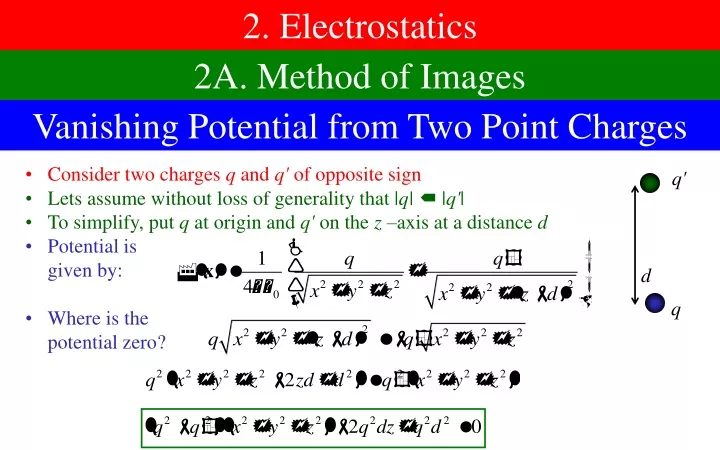
1. 2. Electrostatics 2A. Method of Images Vanishing Potential from Two Point Charges • Consider two charges q and q' of opposite sign • Lets assume without loss of generality that |q| |q'| • To simplify, put q at origin and q' on the z –axis at a distance d • Potential isgiven by: • Where is thepotential zero? q' d q

2. Case 1: Planes • Suppose the two charges are equal andopposite, then the potential vanishes at • This is a plane that is equidistant between the two points How is this useful? • Suppose we have a plane with Dirichletboundaryconditions  = 0 on the plane • If you pretend there is an “image charge” – q on the other sideof the Dirichlet boundary, the two charges will produce a potentialthat cancels on the boundary • It will also satisfy 2 = –/0 in the allowed region –q d q

3. Sample Problem 2.1 (1) An infinite line of charge with linear charge density  is at z = h, x = 0 above a plane conductor at z = 0. Find the electric field everywhere for z > 0, and the surface charge. • The conductor is at constant potential • Since it extends forever, assume it has  = 0 • Add an opposite charge line charge on the other side of the conductor • This guarantees that  = 0 on the conductor • Electric field from the original line charge •  is a vector pointing from the linecharge directly to the point of interest • So the electric field from the original line is • The image line charge causes an electric field • So the total field is:

4. Sample Problem 2.1 (2) An infinite line of charge with linear charge density  is at z = h, x = 0 above a plane conductor at z = 0. Find the electric field everywhere for z > 0, and the surface charge. • To find the surface charge on the conductor, first find the electric field there • Note that it is perpendicular to the surface there, as it must be • Related to surface density by • Can show that, in this case, integrated surface charge cancels the original line

5. Case 2: Spheres • Suppose |q| > |q'|then the potentialvanishes when • Complete the square • This is a sphere of radius: • Distance from q to center: • Distance from q' to center: a r' q' r d q

6. Conducting Spheres a • Let’s put these formulastogether in a useful way: How is this useful? • Suppose we had a grounded ( = 0) conducting sphere of radius a • Plus a point charge q at distance r > a • Pretend there is an imagecharge q' at distance r', where • This will exactly cancel the potential fromthe charge q on the surface of the sphere • And it will satisfy 2 = 0 outside the sphere • So we have solved the problem! r' q' r q

7. Sample Problem 2.2a A conducting sphere of radius a with potential  = 0 at the origin has a charge q on the z-axis at z = 2a. Find the potential (outside), and the total charge on the sphere. q • Add an image chargeof magnitude • It will be at • The potential is then To get the charge: • The hard way: • Find the electric field from the potential • Get the surface charge everywhere and integrate • The easy way: • Use Gauss’s Law on a surface surrounding the sphere • Electric field looks like point charge –q/2 • So charge on sphere must be –q/2 2a – q/2 a/2 a

8. Sample Problem 2.2b A neutral conducting sphere of radius aat the origin has a charge q on the z-axis at z = 2a. Find the potential. q • First guess: We can do this exactly the same way as Problem 2.2a • This is wrong because the sphere had charge – q/2 • So far we have  = 0 on the sphere • To cancel this charge, add additional charge + q/2 on the sphere • It will distribute itself uniformly over the surface • This creates additional potential that looks like a point chargeof magnitude + q/2 at the center • Total potential (outside) is sum of these three contributions 2a – q/2 a/2 a q/2

9. Hollow Spheres • We can use the same formulas for spherical cavity in a conductor • Place an image charge at r' of magnitude q' • Combination will cause vanishing potentialon the interior surface • You don’t have to worry about whethersurrounding conductor is neutral, since excesscharge flows away from interior surface • If you want to make   0 on interior surface,just add a constant to it • It is irrelevant anyway. q q'

10. Green’s Functions for Planes and Spheres • Since we know how to get the potential for a point charge near a conducting plane or sphere we can find the Green’s functions for them • Green’s functions (with Dirichlet boundary conditions) satisfy • For a plane at z = 0 for the region z > 0,one source at x, one at xR = (x, y,–z) • For a sphere at origin with radius a, one point at x of size 1, one point at xR = a2x/x2 with magnitude –a/|x| • With some workcan rewrite this as • This formula also works for interior of a sphere as well

11. Using Green’s Functions for Spheres (1) • Probably easiestto use inspherical coordinates •  is anglebetween x and x' • We can then use this formula for Dirichlet problems with spherical boundary • The normal derivative is: • On thesurfacer' = athis becomes

12. Using Green’s Functions for Spheres (1) • Finally, the surface integral will take the form: • So we have

13. Sample Problem 2.3 (1) The potential on the surface of a sphere of radius a centered at the origin is given by  = Ez. Find the potential outside the sphere. x z • We use ourformula forthe potential,ignoring the  term • For purposes of this integral, treat x as if it were the z-axis • This makes  = ' • With this choice of z-axis, what we normally call z-direction becomes •  is angle between x and ordinary z-axis • We are on the surfaceof the sphere, so • So we have: • Set up the integrals

14. Sample Problem 2.3 (2) The potential on the surface of a sphere of radius a centered at the origin is given by  = Ez. Find the potential outside the sphere. x z • Do the ' integral • Let

15. Sample Problem 2.4 A neutral conducting sphere of radius a is placed in a background electric field given by . Find the potential everywhere outside the sphere. • Recall: • This suggests • But this can’t be right because it is not constant at r = a • Let’s try to find a solution of the form: • Since there’s no charge outside, we must have • We need to cancel the potential from the first term, so • We already solved this problem: • So the answer is:

16. 2B. Orthogonal Functions and Expansions General Theory of Orthogonal Functions • Let Un(x) be a set of functions in some region in d dimensions • d may be less than 3, even if the problem is 3-dimensional! • If we have enough functions Un(x), we can often approxi-mate any function as linear combinations of these functions • Often, finite sum is a good approximation for the infinite • It is useful to normally arrange the Un’s to be orthogonal • This can always be arranged • See quantum notes for details • Assuming the integral is finite when m = n, you cannormalize them to make them orthonormal • Given f(x), it is not hard to find the coefficients an:

17. Completeness Relation, and Other Comments • Substitute the expressionon the right into the left • Since this is true for any function f(x),we must have the completeness relation • I’m not sure what  means, because I’m not sure how many dimensions we’re in Sometimes, we might not want all possible functions • We might want functions that vanishat certain locations, so we’d choose • Completeness still works in interior • We might want functions that havevanishing Laplacian, so we’d choose • This will ruin completeness

18. 1D Discrete Fourier Transforms • Consider functions on the region (0, a) with periodic boundary conditions, f(0) = f(a) • It is well known that a complete set of functionsthat satisfy this equation are the Fourier modes: • n =0, 1, 2, 3,  • These are not quite orthonormal • Any function can be written in terms of them: • Coefficients are • Sometimes, it is easier to work with real functions • n = 0, 1, 2, 3,  • Then we can write anyfunction in terms of them: • Coefficients are:

19. 1D With Vanishing Boundaries • If we instead demand that f(0) = 0 = f(a), we should use some different functions • Use real functions, but want them to vanish at these points: • n = 1, 2, 3,  • Not quite orthonormal • We can write an arbitrary function in the form: • The coefficients are given by

20. 2D With Vanishing Boundaries • Suppose we have a 2D problem with f(x,y) where 0 < x < a and 0 < y < b • Let’s suppose we want f to vanish on all four boundaries • Since f vanishes at x = 0 and x = a, we must be able to write • Since f vanishes at y = 0 and y = b, the same must be true of An • Therefore, An must be writable in the form • We therefore have • Coefficients are: b a

21. Continuous Bases • It is sometimes the case that you need to use a basis where n takes on continuous values • We might write the basis functions as U(x) • Then all sums become integrals • The relations above get changed to:

22. Continuous Fourier Transforms • Theorem from quantum: • Consider the set of functions: • They are orthonormal: • Also complete • So we can write arbitraryfunctions in terms of these • Amplitude is given by • Can find similar formulas in 3D:

23. Decomposition in Different Coordinates Consider the Laplacian in 3D in different coordinate systems: • Cartesian: • Cylindrical: • Spherical: • Often good to solve problem explicitly by writing function as a complete function in some of these variables, and unknown function in others

24. 2C. Solving Problems in Cartesian Coordinates The Method • Suppose, for example, you have a boxwith potential zero on some surfaces • And let’s say it’sspecified on others • Write the potential in terms of complete functions on x and y • If there is no charge inside, then

25. Modes That Satisfy Laplace’s Equation • Substitute thisinto Laplace’sequation: • Since these wave functions areindependent, we must have • Define • Then we have • The general solution of this equation is

26. Matching the Boundary Equations • We haven’t matched the boundary conditions • On the top and bottom, we can also write the (known) potential as • We can get thecoefficients • To get it to match at z = 0, we must have • To get it to match at z = c, we must have • Two equations in two unknowns • Solve for nmand nm and we have 

27. Sample Problem 2.5 (1) A cube of size a has potential 0 on five faces and potential  = xy on the last face. What is the potential everywhere, and at the center? • We have • We need it to vanish on z = 0, so nm = –nm • To match on z = a,we have • Find thecoefficients

28. Sample Problem 2.5 (2) A cube of size a has potential 0 on five faces and potential  = xy on the last face. What is the potential everywhere, and at the center? • Now just substitute in the center

29. 2D. Solving Probs. in Cylindrical Coordinates Potential in a Sharp Corner • Laplacian in cylindrical coordinates • Let’s do a 2D problem • Everything independent of z • Consider a sharp conducting angle of size  with vanishing potential • Presumably other sources/potentials somewhere else • The potential must vanish at  = 0 and  =  • We therefore canwrite the potential as • Substitute into • To make this vanish, we must have 

30. Solving the Radial Equation • Second order differential equation shouldhave two linearly independent solutions • Guess solutions of the form • We therefore have • We therefore have • The general solution is • If we want finite potential near  = 0, must choose Bn = 0 • Therefore: • Largest contribution from n = 1:

31. Electric Field near a Sharp Corner • The electric field is the derivative of the potential • This expression diverges at small  if >  • The sharper the corner, the faster it diverges • In 3D, electric fields maximum at pointy places • Lightning rods have large fields, cause charge to flow from atmosphere • Drains away charge buildup in vicinity of the rod 