Download
1 / 33
360 likes | 471 Views
Smooth Sensitivity and Sampling. CompSci 590.03 Instructor: Ashwin Machanavajjhala. Project Topics. 2-3 minute presentations about each project topic . 1-2 minutes of questions about each presentation. Recap: Differential Privacy. For every pair of inputs that differ in one value.

E N D
Smooth Sensitivity and Sampling CompSci 590.03Instructor: AshwinMachanavajjhala Lecture 7 : 590.03 Fall 12
Project Topics • 2-3 minute presentations about each project topic. • 1-2 minutes of questions about each presentation. Lecture 7 : 590.03 Fall 12
Recap: Differential Privacy For every pair of inputs that differ in one value For every output … D1 D2 O Adversary should not be able to distinguish between any D1 and D2 based on any O Pr[A(D1) = O] Pr[A(D2) = O] . log < ε (ε>0) Lecture 7 : 590.03 Fall 12
Recap: Laplacian Distribution Database Query q True answer q(d) q(d) + η Researcher Privacy depends on the λ parameter η h(η) α exp(-η / λ) Mean: 0, Variance: 2 λ2 Lecture 7 : 590.03 Fall 12
Recap: Laplace Mechanism [Dwork et al., TCC 2006] Thm: If sensitivity of the query is S, then the following guarantees ε-differential privacy. λ = S/ε Sensitivity: Smallest number s.t. for any d, d’ differing in one entry, || q(d) – q(d’) || ≤ S(q) Lecture 7 : 590.03 Fall 12
Sensitivity of Median function • Consider a dataset containing salaries of individuals • Salary can be anywhere between $200 to $200,000 • Researcher wants to compute the median salary. • What is the sensitivity? Lecture 7 : 590.03 Fall 12
Queries with Large Sensitivity • Median, MAX, MIN … • Let {x1, …, x10} be numbers in [0, Λ]. (assume xi are sorted) • qmed(x1, …, x10) = x5 Sensitivity of qmed = Λ • d1 = {0, 0, 0, 0, 0, Λ, Λ, Λ, Λ, Λ} – qmed(d1) = 0 • d2 = {0, 0, 0, 0, Λ, Λ, Λ, Λ, Λ, Λ} – qmed(d2) = Λ Lecture 7 : 590.03 Fall 12
Minimum Spanning Tree • Graph G = (V,E) • Each edge has weight between 0, Λ • What is Global Sensitivity of cost of minimum spanning tree? • Consider complete graph with all edge weights = Λ. Cost of MST = 3Λ • Suppose one of the edge’s weight is changed to 0Cost of MST = 2Λ Λ Λ Λ 0 Λ Λ Lecture 7 : 590.03 Fall 12
k-means Clustering • Input: set of points x1, x2, …, xn from Rd • Output: A set of k cluster centers c1, c2, …, ck such that the following function is minimized. Lecture 7 : 590.03 Fall 12
Global Sensitivity of Clustering Lecture 7 : 590.03 Fall 12
Queries with Large Sensitivity • However for most inputs qmed is not very sensitive. x4 ≤ qmed(d’) ≤ x6 Sensitivity of qmed at d = max(x5 – x4, x6 – x5) << Λ d x1 x2 x3 x4 x5 x6 x7 x8 x9 x10 d’ x1 x2 x3 x4 x5 x6 x7 x8 x9 x10 Λ 0 d’ differs from d in k=1 entry Lecture 7 : 590.03 Fall 12
Local Sensitivity of q at d – LSq(d) [Nissim et al., STOC 2007] Smallest number s.t. for any d’ differing in one entry from d, || q(d) – q(d’) || ≤ LSq(d) Sensitivity = Global sensitivity S(q) = maxdLSq(d) Can we add noise proportional to local sensitivity? Lecture 7 : 590.03 Fall 12
Noise proportional to Local Sensitivity • d1 = {0, 0, 0, 0, 0, 0, Λ, Λ, Λ, Λ} • d2 = {0, 0, 0, 0, 0, Λ, Λ, Λ, Λ, Λ} differ in one value Lecture 7 : 590.03 Fall 12
Noise proportional to Local Sensitivity • d1 = {0, 0, 0, 0, 0, 0, Λ, Λ, Λ, Λ} qmed(d1) = 0 LSqmed(d1) = 0 => Noise sampled from Lap(0) • d2 = {0, 0, 0, 0, 0, Λ, Λ, Λ, Λ, Λ} qmed(d2) = 0 LSqmed(d2) = Λ => Noise sampled from Lap(Λ/ε) • Pr[answer > 0 | d2] > 0 • Pr[answer > 0 | d1] = 0 • Pr[answer > 0 | d2] > 0 • Pr[answer > 0 | d1] = 0 = ∞ • implies Lecture 7 : 590.03 Fall 12
Local Sensitivity LSqmed(d1) = 0 & LSqmed(d2) = Λ implies S(LSq(.)) ≥ Λ LSqmed(d) has very high sensitivity. Adding noise proportional to local sensitivity does not guarantee differential privacy Lecture 7 : 590.03 Fall 12
Sensitivity Local Sensitivity Global Sensitivity Smooth Sensitivity D1 D2 D3 D4 D5 D6 Lecture 7 : 590.03 Fall 12
Smooth Sensitivity [Nissim et al., STOC 2007] S(.) is a β-smooth upper bound on the local sensitivity if, For all d, Sq(d) ≥ LSq(d) For all d, d’ differing in one entry,Sq(d) ≤ exp(β) Sq(d’) • The smallest upper bound is called β-smooth sensitivity. S*q(d) = maxd’ ( LSq(d’) exp(-mβ) ) where d and d’ differ in m entries. Lecture 7 : 590.03 Fall 12
Smooth sensitivity of qmed • x5-k ≤ qmed(d’) ≤ x5+k • LS(d’) = max(xmed+1 – xmed, xmed – xmed-1) S*qmed(d) = maxk (exp(-kβ) x max 5-k ≤med≤ 5+k(xmed+1 – xmed, xmed – xmed-1)) d x1 x2 x3 x4 x5 x6 x7 x8 x9 x10 d’ x8 x9 x10 Λ Λ Λ 0 0 0 x1 x2 x3 x4 x5 x6 x7 d’ differs from d in k=3 entries Lecture 7 : 590.03 Fall 12
Smooth sensitivity of qmed For instance, Λ = 1000, β = 2. S*qmed(d) = max ( max0≤k≤4(exp(-β∙k) ∙ 1), max5≤k≤10 (exp(-β∙k) ∙ Λ) ) = 1 d 1 2 3 4 5 6 7 8 9 10 Lecture 7 : 590.03 Fall 12
Calibrating noise to smooth sensitivity Lecture 7 : 590.03 Fall 12
Calibrating noise to smooth sensitivity Theorem • If h is an (α,β) admissible distribution • If Sqis a β-smooth upper bound on local sensitivity of query q. • Then adding noise from h(Sq(D)/α) guarantees: P[f(D) O] ≤ eεP[f(D’) O] + δfor all D, D’ that differ in one entry, and for all outputs O. Lecture 7 : 590.03 Fall 12
Calibrating Noise for Smooth Sensitivity A(d) = q(d) + Z ∙ (S*q(x) /α) • Z sampled from h(z) 1/(1 + |z|γ), γ > 1 • α = ε/4γ, • S* is ε/γ smooth sensitive • P[f(D) O] ≤ eε P[f(D’) O] Lecture 7 : 590.03 Fall 12
Calibrating Noise for Smooth Sensitivity • Laplace and Normally distributed noise can also be used. • They guarantee (ε,δ)-differential privacy. Lecture 7 : 590.03 Fall 12
Summary of Smooth Sensitivity • Many functions have large global sensitivity. • Local sensitivity captures sensitivity of current instance. • Local sensitivity is very sensitive. • Adding noise proportional to local sensitivity causes privacy breaches. • Smooth sensitivity • Not sensitive. • Much smaller than global sensitivity. Lecture 7 : 590.03 Fall 12
Computing the (Smooth) Sensitivity • No known automatic method to compute (smooth) sensitivity • For some complex functions it is hard to analyze even the sensitivity of the function. Lecture 7 : 590.03 Fall 12
Sample and Aggregate Framework Sample without replacement Original Data ( ) Original Function New Aggregation Function Lecture 7 : 590.03 Fall 12
Example: Statistical Analysis [Smith STOC’11] • Let T be some statistical point estimator on data (assumed to be drawn i.i.d. from some distribution) • Suppose T takes values from [-Λ/2, Λ/2], sensitivity = Λ Solution: • Divide data X into K parts • Compute T on each of the K parts: z1, z2, …, zK • Compute (z1, z2, …, zK)/K Lecture 7 : 590.03 Fall 12
Example: Statistical Analysis [Smith STOC’11] Solution: • Divide data X into K parts • Compute T on each of the K parts: z1, z2, …, zK • Compute : AveK,T = (z1, z2, …, zK)/K Utility Theorem: Lecture 7 : 590.03 Fall 12
Example: Statistical Analysis [Smith STOC’11] Solution: • Divide data X into K parts • Compute T on each of the K parts: z1, z2, …, zK • Compute : AveK,T = (z1, z2, …, zK)/K Privacy: Average is a deterministic algorithm. So does not guarantee differential privacy. (Add noise calibrated to sensitivity of average) Lecture 7 : 590.03 Fall 12
Widened Windsor Mean • α-Windsorized Mean: W(z1, z2, …, zk) • Round up the αk smallest values to zαk • Round down the αk largest values to z(1-α)k • Compute the mean on the new set of values. • If statistician knows a = z(1-α)kand b = zαk • Sensitivity = |a-b|/kε • If not known, a and b can be estimated using exponential mechanism. Lecture 7 : 590.03 Fall 12
Summary • Local sensitivity can be much smaller than global sensitivity • But local sensitivity may be a very insensitive function. • Need to use a smooth upperbound on local sensitivity • Sample and Aggregate framework helps apply differential privacy when computing sensitivity is hard. Lecture 7 : 590.03 Fall 12
Next Class • Optimizing noise when a workload of queries are known. Lecture 7 : 590.03 Fall 12
References C. Dwork, F. McSherry, K. Nissim, A. Smith, “Calibrating noise to sensitivity in private data analysis”, TCC 2006 K. Nissim, S. Raskhodnikova, A. Smith, “Smooth Sensitivity and sampling in private data analysis”, STOC 2007 A. Smith,"Privacy-preserving statistical estimation with optimal convergence rates", STOC 2011 Lecture 7 : 590.03 Fall 12