Download
1 / 15
150 likes | 242 Views
Toy Monte Carlo for the Chromatic Correction in the Focusing DIRC Data. Jose Benitez 8/29/2006. Outline . Compare Resolutions of Focusing DIRC with BaBar DIRC. Toy Monte Carlo:

E N D
Toy Monte Carlo for the Chromatic Correction in the Focusing DIRC Data Jose Benitez 8/29/2006
Outline • Compare Resolutions of Focusing DIRC with BaBar DIRC. • Toy Monte Carlo: • In this example photons will be generated from beam position 1 in bar and the SOB path length will not be taken into account. • Reconstruct using ultimate Focusing DIRC resolutions (using 6x6mm pixels). • Apply Method1 of b resolution calculation. • Show results as function of photon path length. • Show new method (Method2) of calculating b resolution.
Resolution Comparison With BaBar DIRC Angular (q) Resolution • Pixel Size resolution is for 6x6mm pads (slot4). • Chromatic Smearing is irrelevant in this model. • Path length resolution depends both q and f resolution. Timing Resolution Photon Path Length Resolution
Photon Track Description ˆ n PMTs mirror q z0 b lb The photon track is fully described by the following variables. z0 , n , b, l, q, j, L, v, T not all independent. ˆ • In this toy Monte Carlo I specialize to photons with the following parameters: • z0 for beam position 1 • n normal to the bar. • b=1 for 10GeV electrons • j fixed for indirect photons traveling straight down the bar, so no side bounces • only up down bounces. These parameters are adequate for photons detected in slot 4. ˆ We are left with the following variables to vary: l, q, L, v, T
Wavelength Generation: l 1. Determine wavelength distribution at production. 2. Find all wavelength dependent efficiencies in the detector. 3. Multiply above distributions to get final distribution.
l in mm in this formula. Generation of Theta q mean=1.4697 rms=.0059 • The Angle q at which the photons are produced is given by the Cherenkov equation: where b=1 and n(l) is the index of refraction of the bar: mean=822mrad rms=3.7mrad
Generation of Photon Speed: v mean=1.5139 rms=.0196 • The speed of a photon with a given wavelength traveling inside the bar is given by: where mean=.6607 rms=.0085
Generation of the Photon Path Length L and Propagation Time T • Given that the particle track is perpendicular to the bar and that we are considering photons traveling straight down the bar, the total path length for indirect (mirror reflected) photons is given by: • Finally the propagation time is given by: mean=9.2m rms=.032m mean=46.5ns rms=.4396ns
Reconstruction: mean=9.2m rms=.098m mean=46.5ns rms=.4509ns • With the Focusing DIRC we are able to measure the following observables : q , L , T from which we can calculate the necessary quantities: q, v mean=822mrad rms=7.7mrad mean=.6607 rms=.0109 • Monte Carlo • _ PDF Projection • Monte Carlo • _ PDF Projection
Correlation of q with v Distribution with sq=.5mrad, sv /c0=.5e-3 l Efficiency Off (300nm<l<650nm) Distribution with sq=.5mrad, sv /c0=.5e-3 l Efficiency On PDF used in this Toy Monte Carlo to calculate b. b is varied between .93 and 1.07. sq=6.8mrad sv /c0=1.5e-3 l Efficiency On This Toy Monte Carlo
Results: sb=7.74e-3 This Example: sq=6.8mrad sT=100ps sL / L=1% L~9.2m BaBar DIRC As Function of L: sq=6.8mrad Focusing DIRC For explanation of Method2 see later slides. These numbers are equivalent to ones obtained using Method1.
Conclusions • This toy Monte Carlo shows that this method of reconstructing our data actually works. • The path length error is actually taking a significant amount of chromatic correction; about half of it. However there is not much we can do about, this error is determined by the pixel size as well as other angular smearing.
Method 2 of b Resolution Calculation • Suppose you had a detector fixed at some angle q0 and which could only detect photons with speed v0. Also assume this detector has errors in the measurements of q0 and v0 equal to sq and sv respectively. Consider the following question: • What is the b of the particle which produced your measurements? • Answer: As you might expect there is not a unique b which produced your measurements because you have errors. Rather there is a distribution of b’s which can generate (q0,v0 ), this distribution of b’s is given by the PDF evaluated at q=q0 and v=v0: PDF(b,q=q0,v=v0). • Comments: • In this method we are using the PDF in “reverse mode”. Earlier I used the PDF with fixed b=1 to generate a 2D distribution which describes our measurements of q and v, now I am doing the opposite. I know, for example that q=822mrad and v=.66c corresponds to b=1, so I can use the PDF to generate a Gaussian distribution centered at b=1, the sigma of this distribution is non other than the b resolution of a detector which can measure q an v with resolutions sq and sv. • This method provides a very quick way of calculating the b resolution. In fact the b resolutions in the previous slides (as a function of path length) were calculated using this method, Method1 is very time consuming. • I believe what is going on behind this method is that we are just projecting the PDF onto the b axis.
Example: sb=7.78e-3 This Example: sq=6.8mrad sT=100ps sL / L=1% L~9.2m q0=.822mrad v0=.66c As Function of L: sq=6.8mrad sT=100ps sL / L=1% q0=.822mrad v0=.66c The small differences (~.6%) can be caused by statistics and/or fit errors.