Download
1 / 25
250 likes | 541 Views
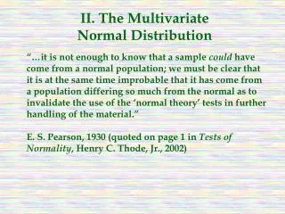
Statistical Analysis – Chapter 4 Normal Distribution . What is the normal curve?. In chapter 2 we talked about histograms and modes

E N D
What is the normal curve? • In chapter 2 we talked about histograms and modes • A normal distribution is when a set of values for one variable, when displayed in a histogram (or line graph) has one peak (mode) and looks like a bell. Here is an example using height:
Characteristics of the Normal Curve • Bell shaped, fading at the tails. In other words, more values are in the middle, and odd or unusual values fall at the tails • All (100%) of the data fits on the curve, with 50% before the mean and 50% after • 68% of the data falls within -1 and +1 standard deviations of the mean • 95% of the data falls between -2 and +2 standard deviations • The percentage of data between any two points is equal to the probability of randomly selecting a value between the two points (remember classical probability from Ch. 3)
Standard Deviations and Z-Score • Z – scores = the number of standard deviations away from the mean. • z-score = x - µ σ (x = data for which we want to know the z-score) • We use the characteristics of the normal curve, and the z-score, to find out the probability of a particular event or value occurring (remember classical probability from Chapter 3)
Solving Normal Curve Problems Using Z-Scores (steps listed at bottom of p. 111) • Draw a normal curve, showing values for (-2 through +2) • Shade the area in question • Calculate the z scores and cutoffs (percentages asked for) • Use the z-scores and cutoffs to solve the normal curve problem
Find Percentages on the Normal Curve Table Let’s do these questions as a class… • What is the percentage of data from z = 0 to z = 0.1? • What is the percentage of data from z = 0 to z = 2.16? • What is the percentage of data from z = -1.11 to z = 1.11? • What is the percentage of data above z = 1.24? • What is the percentage of data below z = -0.6? Answers • .0398…39.8% • .4846…48.46% • .3665 + .3665 = .733…73.3% • .50 - .3925 = .1075…10.75% • .50 - .2257 = .2743…27.43%
Working backwards from percentages… • When working backwards from percentages, we still use the normal table…but look for the percentage to give us the z-score… • What is the z-score associated 10.2% of the data? • What is the z-score(s) for the middle 30% of the normal curve? • What is the z-score of data in the upper 25% of the normal curve? Answers • z = 0.26 • z = -.39 to z = .39 • z = 0.67
Let’s do Question 4.2 Use the normal curve table to determine the percentage of data in the normal curve • Between z = 0 and z = .82 • Above z = 1.15 • Between z = -1.09 and z = .47 • Between z = 1.53 and z = 2.78 Work backward in the normal curve table to solve the following: • 32% of the data in the normal curve data can be found between z = 0 and z = ? • Find the z score associated with the lower 5% of the data. • Find the z scores associated with the middle 98% of the data.
Question 4.2 Answers Answers to Question 4.2 • 29.39% • 12.51% • 54.29% • 6.03% • Between z = 0 and z = .92, or between z = 0 and z = -.92
Question 4.7 Use the normal curve table to determine the percentage of data in the normal curve • Between z = 0 and z = .38 • Above z = -1.45 • Above z = 1.45 • Between z = .77 and z = 1.92 • Between z = -.25 and z = 2.27 • Between z = -1.63 and z = -2.89 Work backward in the normal curve table to solve the following. • 15% of the data in the normal curve can be found between z = 0 and z = ? • Find the z score associated with the upper 73.57% of the data. • Find the z scores associated with the middle 95%
Question 4.7 Answers • 14.80% • 92.65% • 7.35% • 19.32% • 58.71% • 4.97% • z = .39 or -.39 • z = -.63 • Between z = -1.96 and z = +1.96
Binomial Distributions and Sampling Binomial means two categories in a population… • Males and females • Sports game players vs. Non sports game players • Incomes over 40,000 vs. incomes under 40,000 Quick note: Remember…for binomial distributions, we would visualize this data through a pie chart…because we do not have enough categories for a histogram…
Sampling from a Two-Category Population • With two-category populations, we can describe the population by p – the percentage of values in one category • This is the same p from the last chapter on probability (classical probability)… P(event) ≈ s (number of chances for success) n (total equally likely possibilities) • We know (actually….statisticians know) that if we randomly sampled from a population, then ps ≈ p
Sampling Distribution • In order to know the odds of getting certain values from this particular binomial sample, we have to know the sampling distribution from this population. • Under certain conditions, the sampling distribution for a binomial value is normal (i.e. the distribution follows the normal curve). • When the sampling distribution is normal, then we can make predictions using our table and our z-scores
Sampling from a Binomial Distribution • Suppose, we defined a population (full time FIT students who either shop at Hot Topic), and we have made our measure of interest into a binomial distribution – those who shop at Hot Topic and those who do not. • Suppose over the last 10 years, marketers have surveyed the FIT population hundreds of times and found that Hot Topic shoppers are p = .13. (those who are non-Hot Topic shoppers is p = .87)
Sampling from a Binomial Distribution • But suppose sometime later, your manager asks you to lead another study. But this time, you don’t have enough money to survey the whole population, and you have to get a sample. • We can assume, because so many studies have been done in the past that the true value of Hot Topic shoppers is p = .13. Thus, because we know that ps ≈ p, your sample should have approximately the same value.
Sampling from a Binomial Distribution • For each sample, we can use the number sampled, and the p value from the population to predict the total number of Hot Topic shoppers. This is called the expected value. • Expected value = np • Thus, if we collected a sample of 200 FIT students, how many students would we expect to be Hot Topic shoppers? np = (200)(.13) = 26 • This expected value is the mean of your sample
Binomial Distribution and the Normal Curve • Now, we need to decide if we can use the normal curve to solve problems… • If (np) > 5 and n(1 – p)>5…then the sampling distribution will be normally distributed. • So, our sample was 200 students. Is (np) > 5? Is n(1 – p)>5? • Yes…and yes. np = (200)(.13) = 26 n(1 – p) = (200)(1 - .13) = (200)(.87) = 174
Binomial Distribution and the Normal Curve • What do we mean that a sampling distribution is normal? • Just like someone’s age is one value among many ages that we tally to make a histogram, we can tally many samples, get the p values of those sample, and construct histograms from these means. • If we took say, 1000 samples, and tallied the p values for Hot Topic shoppers, then those values, when turned into a histogram, should form a normal curve. Just like if we took the heights of a 1000 women, and tallied those values to get a normal curve.
How to use the Binomial Distribution and the Normal Curve • Get the mean (µ)…the mean is the expected value (np) • Get the standard deviation (σ) = √np(1 – p) • Draw a normal curve using mean and standard dev • Use the “continuity correction factor,” and add +/- half a unit to the value we want to solve for • Get the z-scores = x - µ σ • Use the normal curve table to solve the problem
Why the “continuity correction factor”? • This is only for discrete values (where values occupy only distinct points.) For example, in our study, there is no such thing as a “half” or “3/4” Hot Topic shopper. Either you are a shopper or not. Looking at how histograms are presented, you can see why we have to use the correction factor. • Probability of getting a value equal to or greater than (=>), then you must subtract a half-unit • Probability of getting a value equal to or lesser than (=<), you must add a half unit. • Probability of getting the exact value, you must get the Z-scores for a half-unit above and a half-unit below
Now let’s answer a Hot Topic Question… If you collected a sample of 200 FIT students… • What is the probability that 13 will be Hot Topic shoppers? • What is the probability that you will have 30 or more Hot Topic shoppers? • What is the probability that you will have 25 or less Hot Topic shoppers?
Question • What is the probability that 13 will be Hot Topic shoppers? • What is the probability that you will have 30 or more Hot Topic shoppers? • What is the probability that you will have 25 or less Hot Topic shoppers? Answer • Get the mean (µ) = expected value = np = (200)(.13) = 26 • Get the standard deviation (σ) = √np(1 – p) = √26(1 - .13) = √26(.87) = √22.62 ≈ 4.76 • Draw a normal curve using mean and standard dev. • Use the continuity correction factor to correct x. (a) 12.5 and 13.5, (b) 29.5, (c) 25.5 • Get the z-scores. (a) -2.83 and -2.62, (b) .735, (c)-.105 • Solve the problem… (a) 4977 - .4956 = .002, or 2% (b) .50 - .2704 ≈ .23, or 23%, (c) .50 - .0596 = .4404
Now let’s do question 4.16 as a class… In a marketing population of phone calls, 3% produced a sale. If this population proportion (p = 3%) can be applied to future phone calls, then out of 500 randomly monitored phone calls, • How many would you expect to produce a sale? • What is the probability of getting 11 to 14 sales? • What is the probability of getting 12 or less sales? • 15 • 32.93% • 25.46%
Question 4.16 answers • Expected value = np = 500(.03) = 15 • 32.93% • 25.46%