Download
1 / 60
650 likes | 1.15k Views
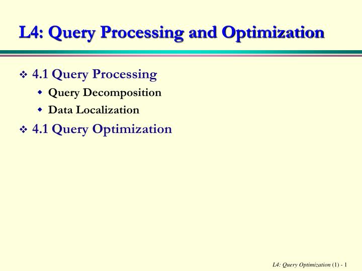
L4: Query Processing and Optimization. 4.1 Query Processing Query Decomposition Data Localization 4.1 Query Optimization. Query Processing. Any high-level query (SQL) on a database must be processed, optimized and executed by the DBMS

E N D
L4: Query Processing and Optimization • 4.1 Query Processing • Query Decomposition • Data Localization • 4.1 Query Optimization
Query Processing • Any high-level query (SQL) on a database must be processed, optimized and executed by the DBMS • The high-level query is scanned, and parsed to check for syntactic correctness • An internal representation of a query is created, which is either a query tree or a query graph • The DBMS then devises an execution strategy for retrieving the result of the query. (An execution strategy is a plan for executing the query by accessing the data, and storing the intermediate results) • The process of choosing one out of the many execution strategies is known as query optimization
Query Processor • A query processor is a module in the DBMS that performs the tasks to process, to optimize, and to generate execution strategy for a high-level query • For a DDBMS, the QP also does data localization for the query based on the fragmentation scheme and generates the execution strategy that incorporates the communication operations involved in processing the query
Query Optimizer • Queries expressed in SQL can have multiple equivalent relational algebra query expressions • The distributed query optimizer must select the ordering of relational algebra operations, sites to process data, and possibly the way data should be transferred. This makes distributed query processing significantly more difficult
Complexity of Relational Algebra Operations • The relational algebra is used to express the output of the query. The complexity of relational algebra operations play a role in defining some of the principles of query optimization. All complexity measures are based on the cardinality of the relation • Operations Complexity Select, Project (w/o duplicate elimination) O(n) Project (with duplicate elimination), Group O(n logn) Join, Semi-join, Division, Set Operators O(n logn) Cartesian Product O(n2 ) This was given in the book (p194). It is over simplified.
Characteristics of Query Processors • Statistics • fragment cardinality and size • size and number of distinct values for each attribute. detailed histograms of attribute values for better selectivity estimation. • Decision Sites • one site or several sites participate in selection of strategy • Exploitation of network topology • wide area network communication cost • local area network parallel execution
Characteristics of Query Processors • Exploitation of replicated fragments • larger number of possible strategies • Use of Semijoins • reduce size of data transfer • increase # of messages and local processing • good for fast or slow networks?
STATISTICS ON FRAGMENTS GLOBAL SCHEMA FRAGMENT SCHEMA LOCAL SCHEMA Layers of Query Processing Calculus Query on Distributed Relations QUERY DECOMPOSITION CONTROL SITE Algebra Query on Distributed Relations DATA LOCALIZATION Fragment Query GLOBAL OPTIMIZATION Optimized Fragment Query With Communication Operations LOCAL SITE LOCAL OPTIMIZATION Optimized Local Queries
Query Decomposition • Normalization • Convert from general language (SQL) to a “standard” form (e.g., Relational Algebra) • Query qualification is written in a normalized form (CNF or DNF) for subsequent manipulation • Analysis • The query is analyzed for syntactic semantic correctness • Simplification • Redundant predicates are eliminated to obtain simplified queries • Restructuring • The calculus query is translated to optimal algebraic query representation
Query Decomposition: Normalization • There are two possible forms of representing the predicates in query qualification: Conjunctive Normal Form (CNF) or Disjunctive Normal Form (DNF) • CNF: (p11 p12... p1n) ... (pm1 pm2... pmn) • DNF: (p11 p12... p1n) ... (pm1 pm2... pmn) • OR's mapped into union • AND's mapped into join or selection • Lexical and syntactic analysis • check validity • check for attributes and relations • type checking on the qualification
Example Select A,C From R,S Where (R.B=1 and S.D=2) or (R.C>3 and S.D.=2) (R.B=1 v R.C>3) S.D.=2 R S A, C Conjunctive normal form
Query Decomposition: Analysis • Queries are rejected because • the attributes or relations are not defined in the global schema; or • operations used in qualifiers are semantically incorrect • For only those queries that do not use disjunction or negation semantic correctness can be determined by using query graph • One node of the query graph represents result sites, others operand relations, edge between nodes operand nodes represent joins, and edge between operand node and result node represents project
Analysis: Detect invalid expressions E.g.: Select * from R where R.A =3 R does not have “A” attribute
PROJ PROJ Result ASG EMP ASG EMP Query Graph and Join Graph SELECT Ename, Resp FROM E, G, J WHERE E. ENo = G. ENO AND G.JNO = J.JNO AND JNAME = ``CAD'' AND DUR >= 36 AND Title = ``Prog'' E. ENo = G. ENO G.JNO = J.JNO Ename JNAME = ``CAD'' Resp Title = ``Prog'' E. ENo = G. ENO G.JNO = J.JNO DUR >= 36
PROJ Result EMP ASG Disconnected Query Graph • Semantically incorrect conjunctive multivariable query without negation have query graphs which are not connected SELECT Ename, Resp FROM E, G, J WHERE E. ENo = G. ENO AND JNAME = ``CAD'' AND DUR >= 36 AND Title = ``Prog'' Ename Resp Title = ``Prog'' E. ENo = G. ENO DUR >= 36 JNAME = ``CAD''
Simplification: Eliminating Redundancy • Elimination of redundant predicates using well known idempotency rules: p p = p; p p = p; p true = true; p false = p; p true = p; p false = false; p1 (p1 p 2 ) = p1; p1 (p1 p 2 ) = p1 • Such redundant predicates arise when user query is enriched with several predicates to incorporate view relation correspondence, and ensure semantic integrity and security
Eliminating Redundancy-- An Example SELECT TITLE FROM E WHERE (NOT (TITLE = ``Programmer'') AND (TITLE = ``Programmer'' OR TITLE = ``Elec.Engr'') AND NOT (TITLE = ``Elec.Engr'')) OR ENAME = ``J.Doe''; SELECT TITLE FROM E WHERE ENAME = ``J.Doe'';
Eliminating Redundancy-- An Example • p1 = <TITLE = ``Programmer''> • p2 = <TITLE = ``Elec. Engr''> • p3 = <ENAME = ``J.Doe''> Let the query qualification is (¬p1 (p1 p2) ¬p2) p3 The disjunctive normal form of the query is = (¬p1 p1 ¬p2) (¬p1 p2 ¬p2) p3 = (false¬p2) (¬p1 false) p3 = falsefalse p3 = p3
Query Decomposition: Rewriting • Rewriting calculus query in relational algebra; • straightforward transformation from relational calculus to relational algebra, and • restructuring relational algebra expression to improve performance
R S S R (R S) T R (S T) Rewriting -- Transformation Rules (I) • Commutativity of binary operations: R S S R R S S R • Associativity of binary operations: (R S) T R ( S T ) • Idempotence of unary operations: grouping of projections and selections • A’ ( A’’ (R )) A’ (R ) for A’A’’ A • p1(A1) ( p2(A2) (R )) p1(A1) p2(A2) (R )
Rewriting -- Transformation Rules (II) • Commuting selection with projection A1, …, An ( p (Ap) (R )) A1, …, An ( p (Ap) (A1, …, An, Ap(R ))) • Commuting selection with binary operations p (Ai)(R S) ( p (Ai)(R)) S p (Ai)(R S) ( p (Ai)(R)) S p (Ai)(R S) p (Ai)(R) p (Ai)(S) • Commuting projection with binary operations C(R S) A(R) B (S) C = A B C(R S) C(R) C (S) C (R S) C (R) C (S)
JNO ENO An SQL Query and Its Query Tree ENAME (ENAME<>“J.DOE” )(JNAME=“CAD/CAM” ) (Dur=12 Dur=24) SELECT Ename FROM J, G, E WHERE G.Eno=E.ENo AND G.JNo = J.JNo AND ENAME <> `J.Doe' AND JName = `CAD' AND (Dur=12 or Dur=24) PROJ ASG EMP
ENO JNO Query Decomposition: Rewriting ENAME JNO, ENAME JNO JNAME=“CAD/CAM” JNO, ENO ENO, ENAME Dur=12 Dur=24 ENAME<>“J.DOE” PROJ ASG EMP
Data Localization Input: Algebraic query on distributed relations • Determine which fragments are involved • Localization program • substitute for each global query its materialization program • optimize
ENO JNO Data Localization-- An Example EMP is fragmented into EMP1 = ENO “E3” (EMP) EMP2 = “E3” < ENO “E6” (EMP) EMP3 = ENO >“E6” (EMP) ENAME Dur=12 Dur=24 ENAME<>“J.DOE” ASG is fragmented into ASG1 = ENO “E3” (ASG) ASG2 = ENO >“E3” (ASG) JNAME=“CAD/CAM” PROJ ASG1 ASG1 ASG2 EMP1 EMP2 EMP3
ENO=“E5” ENO=“E5” ENO=“E5” EMP EMP2 EMP1 EMP2 EMP3 Reduction with Selection EMP is fragmented into EMP1 = ENO “E3” (EMP) EMP2 = “E3” < ENO “E6” (EMP) EMP3 = ENO >“E6” (EMP) SELECT * FROM EMP WHERE ENO=“E5” Given Relation R, FR={R1, R2, …, Rn} where Rj =pj(R) pi(Rj) = if x R: (pi(x)pj(x))
ENO ENO ASG1 ASG1 ASG2 EMP1 EMP2 EMP3 ASG EMP Reduction with join SELECT * FROM EMP, ASG WHERE EMP.ENO=ASG.ENO EMP is fragmented into EMP1 = ENO “E3” (EMP) EMP2 = “E3” < ENO “E6” (EMP) EMP3 = ENO >“E6” (EMP) ASG is fragmented into ASG1 = ENO “E3” (ASG) ASG2 = ENO >“E3” (ASG)
ENO ENO ENO ENO ENO ENO EMP1 ASG1 EMP1 ASG2 EMP2 ASG1 EMP2 ASG2 EMP3 ASG1 EMP3 ASG2 ENO ASG1 ASG1 ASG2 EMP1 EMP2 EMP3 Reduction with Join (I) (R1 R2) S (R1 S) (R2 S)
ENO ENO ENO EMP1 EMP3 EMP2 ASG1 ASG2 ASG2 Reduction with Join (II) Given Ri =pi(R) and Rj =pj(R) Ri Rj = if x Ri , y Rj: (pi(x)pj(y)) Reduction with join 1. Distribute join over union 2. Eliminate unnecessary work
ENAME ENO EMP1 EMP2 Reduction for VF • Find useless intermediate relations Relation R defined over attributes A = {A1, A2, …, An} vertically fragmented as Ri =A’ (R) where A’ A K,D(Ri) is useless if the set of projection attributes D is not in A’ EMP1= ENO,ENAME (EMP) EMP2= ENO,TITLE (EMP) ENAME SELECT ENAME FROM EMP EMP1
EMP1: TITLE=“Programmer” (EMP) EMP2: TITLE“Programmer” (EMP) ASG1: ASG ENO EMP1 ASG2: ASG ENO EMP2 TITLE=“MECH. Eng.” ENO ASG1 ASG1 ASG2 EMP1 EMP2 Reduction for DHF Distribute joins over union Apply the join reduction for horizontal fragmentation SELECT * FROM EMP, ASG WHERE ASG.ENO = EMP.ENO AND EMP.TITLE = “Mech. Eng.”
Selection first TITLE=“Mech. Eng.” TITLE=“Mech. Eng.” TITLE=“Mech. Eng.” TITLE=“Mech. Eng.” ENO ENO ENO ENO ASG1 ASG1 EMP2 ASG2 EMP2 EMP2 EMP2 ASG2 ASG1 ASG2 ASG1 ASG1 ASG1 Reduction for DHF (II) Joins over union
Reduction for HF • Remove empty relations generated by contradicting selection on horizontal fragments; • Remove useless relations generated by projections on vertical fragments; • Distribute joins over unions in order to isolate and remove useless joins
ENAME ENAME ENO=“E5” ENO ENO=“E5” EMP2 EMP1 EMP3 ASG1 EMP2 Reduction for HF --An Example EMP1 = ENO“E4” (ENO,ENAME (EMP)) EMP2 = ENO>“E4” (ENO,ENAME (EMP)) EMP3 = ENO,TITLE (EMP) QUERY SELECT ENAME FROM EMP WHERE ENO = “E5”
Ename resp=”manager” EMP.Eno=ASG.Eno ASG ASG EMP Why Optimization – An Example Query Database EMP(eno, ename, title) ASG(eno, jno, resp, dur) RA tree Query Find the name of the employees who are managing a project? SQL Select ename From EMP e, ASG g Where e.Eno = g. Eno And resp = ‘‘manager’’
ENO ENO ENO resp=“manager” EMP1 resp=“manager” EMP2 ASG1 ASG2 Example - Strategies Plan B Site 5 Fragment Schema resp=“manager” EMP1 = ENO <= 100(EMP) at site 1 EMP2 = ENO > 100(EMP) at site 2 ASG1 = ENO <= 100(ASG) at site 3 ASG2 = ENO > 100(ASG) at site 4 ASG1 ASG2 EMP1 EMP2 Query site: Site 5 Plan A ASG1’ ASG2’
Example – DB Statistics & Costs Database Statistics • EMP has 400 tuples, • ASG has 1000 tuples, • there are 20 managers in ASG • the data is uniformly distributed among sites. • ASG and EMP are locally clustered on attributes RESP and ENO, respectively Costs • tuple access tacc = 1 unit, • tuple transfer ttrans = 10 units,
Costs for Example Plan • The cost of Plan A: Produce ASG’ = 20 tacc = 20 (processing locally) Transfer ASG’ = 20 *ttrans = 200 (transfer to EMP site) Produce EMP’ = (10+10) * tacc* 2 = 40 (join at the EMP site) Transfer EMP’ = 20 * ttrans = 200 (send to Site 5) Total cost = 460 • The cost of Plan B: Transfer EMP = 400 * ttrans = 4,000 (send EMP to Site 5) Transfer ASG = 1000 * ttrans = 10,000 (send ASG to Site 5) Produce ASG’ = 1000 * tacc = 1,000 (selection at Site 5) Join EMP and ASG’ = 400 * 20 * tacc = 8,000 (join at Site 5) Total cost = 23,000
Query Optimization • Problems in query optimization • Determining the physical copies of the fragments upon which to execute the fragment query expressions (also known as materialization) • Selecting the order of execution of operations • Selecting the method for executing each operation • The above problems are not independent, for instance, the choice of the best materialization for a query depends on the order in which operations are executed. But they are treated as independent. Further, • We bypass (1) by taking materialization for granted • We bypass (3) by clustering all operations at the same site as a local database system dependent problem
Query Optimization - Objectives • The selection of alternative query execution strategies is made based on predetermined objectives • Two main objectives: • minimize the total processing time (total cost) • network and computers at nodes do not get loaded. • Response time cannot be guaranteed • minimize the response time • allocation must facilitate parallel execution of the query • but throughput may decrease and cost can be higher than total cost • Total processing time (cost) is the sum of all the time (cost) incurred in executing the query (CPU, I/O, data transfer) • Response time is the elapsed time from the initiation till the completion of the query
Optimization Algorithms – The Issues • Cost model • cost components • weights for each components • costs for primitive operations • Search space • The set of equivalent algebra expressions (query trees) • Search strategies • How do we move inside the search space • Exhaustive search, heuristics, …
Cost Models • The cost measures are: I/O and CPU for centralized DBMSs and I/O, CPU and data transfer costs for DDBMS • Total cost = CPU cost + I/O cost + communication cost • CPU cost: Ccpu* #insts • I/O cost: C i/o* #i/os • Communication Cost Cmsg*#msgs + Ctr*#bytes • Ccpu, C i/o, Ctr and Cmsg are all assumed to be constants. • Response time = sum (sequential operations) • Ccpu*s_#insts • Ci/o*s_#i/os • Cmsg*s_#msg + ctr*s_#bytes • S_x stands for maximum number of sequential x’s that need to be executed to process the query
Intermediate Result Size • The size of the intermediate relations produced during the execution facilitates the selection of the execution strategy • This is useful in selecting an execution strategy that reduces data transfer • The sizes of intermediate relations need to be estimated based on cardinalities of relations and lengths of attributes • R{A1, A2,..., An} fragmented as R1,R2,…, Rn the statistical data collected typically are • len(Ai), length of attribute Ai in bytes • min(Ai) and max(Ai) for ordered domains • card(dom(Ai)) unique values in dom[Ai] • Number of tuples in each fragment card(Rj)
Intermediate Size Estimation • Join selectivity factor SFj(r,s) = card(r * s) / card(r) * card(s) • Selecton selectivity factor SFS(F) = card(F(r)) / card(r) • size(r) = card(r) * len(r) • Cardinality of intermediate relations • SFS(A = value) = 1/card(dom(A)) • SFS(A > value) = max(A) - value/max(A)-min(A) • SFS(A < value) = value - min(A)/max(A)-min(A) • Sfs(p(Ai)p(Aj)) = sfs(p(Ai)) * sfs(p(Aj)) • Sfs(p(Ai) p(Aj)) = sfs(p(Ai)) + sfs(p(Aj)) - sfs(p(Ai)) * sfs(p(Aj)) • SFS(A {values}) = SFS(A = value) * card(values)
Intermediate Size Estimation (II) • Projection card(a(r)) = card(r) • Cartesian product card(r X s) = card(r) * card(s) • Join card(R A=B S) = card(s); if A is key in R, B is foreign key in S card(R A=B S) = SFJ(R,S) * card(r) * card(s) • Union Upper bound = card(r) + card(s) Lower bound = max{card(r), card(s)}
Cost of Processing Primitive Operations • Selection • Projection • Union • Join • nested-loops • sort-merge • hash-based • For distributed join, semi-join is proposed to perform joins
R’=A(R) S R S’ = R’ S R S’ R S S’ Semi-join Amount of data transferred: |R’| + |S’| • join is replaced with a project; followed by semi-join; and then join • the project and join operations are done at one site, and semi-join at another site • amount of data transferred: |R’| + |S’|
Semi-join versus Join • using sem-ijoin increases local processing costs because a relation must be scanned twice (join, project) • For joining intermediate relations produced during semi-join one cannot exploit indices on the base relations • Semi-join may not be good when communication costs are low
EMP PNO,ENO PROJ ENO PNO PNO ASG PROJ ENO ASG EMP Search Space SELECT ENAME, RESP FROM EMP, ASG, PROJ WHERE EMP.ENO=ASG.ENO AND ASG.PNO=PROJ.PNO • Search space is characterized by alternative execution plans • Most optimizers focus on join trees • For N relations, there are O(N!) equivalent join trees ASG EMP PROJ
Restricting Search Space deep tree • O(N!) is large • Considering join methods, the search space is even bigger • Restrict by means of heuristics • Ignore cartisian product • … • Restrict the shape of the join tree • Only consider deep trees • …. R4 R1 R3 R2 bushy tree R4 R3 R1 R2 Left-deep tree R1 R2 R3 R4