Download
1 / 23
320 likes | 1.46k Views
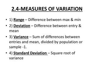
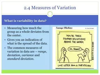
The standard deviation is just the square root of the variance. Measures of Variation. As well as the Central Tendency of the data in a population or sample a second important characteristic of the data is it variability about some center. . Measures of Variation include: The range

E N D
The standard deviation is just the square root of the variance Measures of Variation As well as the Central Tendency of the data in a population or sample a second important characteristic of the data is it variability about some center. • Measures of Variation include: • The range • The Variance • The Standard Deviation • The Mean Absolute Deviation
Measures of Variation Standard Deviation of a Population We will label the population variance to be σ2 And define σ2 = Σi(xi – μ)2/N Where μ is the population mean N is the size of the population Σi(xi – μ)2 is the sum of the squares of the difference between each item in the population and the mean.
Measures of Variation Suppose a student receives the following quiz grades: {82, 68, 74, 86, 90, 88, 62, 75, 80, 55} For this student, these grades are the total population of her scores that are used to calculate her mean or average grade. We obtain: μ = (82 + 68 + 74 + 86 + 90 + 88 + 62 + 75 + 80 + 55)/10 = 760/10 = 76 The mean of this population is 76
Measures of Variation Having obtained the mean, we can now calculate the variance {82, 68, 74, 86, 90, 88, 62, 75, 80, 55} and μ =76 σ2 = Σi(xi – μ)2/N = {(82-76)2 + (68-76)2 + (74-76)2 + (86-76)2 + (90-76)2 + (88-76)2 + (62-76)2 + (75-76)2 + (80-76)2 + (55-76)2 }/10 = (36 + 64 + 4 +100 + 196 + 144 + 196 + 1 + 16 + 441)/10 = 119.8
μ = 76 σ σ Measures of Variation We find the standard deviation in this population data by taking the square root of the variance. σ2 = Σi(xi – μ)2/N = 119.8 σ= (119.8)½ = 10.94 If we display the data on a dot plot, we can visualize the use of the standard deviation as a measure of variation in the data {82, 68, 74, 86, 90, 88, 62, 75, 80, 55} x x x x x x x x x x 55 60 65 70 75 80 85 90 95 100 Mean = 76
Measures of Variation Chebyshev’s Theorem The proportion of any set of data lying within K standard deviations of the mean is always at least 1 – 1/K2, for all K greater than or equal to 2. Chebyshev’s Inequality tells us that in any statistical distribution at least ¾ of the values will lie within 2 standard deviations of the mean, and at least 8/9 of all values will lie within 3 standard deviations of the mean. In the previous example we found μ = 76 and σ= 10.94 μ - 2σ= 76 – 2(10.94) = 54.12 μ + 2σ= 76 + 2(10.94) =97.88 We find that 100% of the values lie within 2σ of the mean
Measures of Variation The Sample Standard Deviation The standard deviation of a sample is denoted by the letter s. The sample standard deviation is an estimate of the population standard deviation σ _ s2 = Σi(xi – x)2/(n – 1) Where x bar in the previous formula denotes the sample mean. The sample standard deviation is obtained by taking the square root of the variance. Note! To calculate the sample variance we divide by the number of degrees of freedom (n – 1) instead of the sample size n. We have already calculated the sample mean when we use the same sample data to obtain a second statistic. Only n-1 of those values are considered free – the nth value is fixed since the sum must equal n times the mean.
Measures of Variation The formula for the standard deviation can be transformed into a form that slightly simplifies the computation. s = (nΣi(xi)2 – (Σixi)2)/n(n – 1))½ On first sight it is not clear that we have simplified the calculation, but if we assume that the previous 10 grades were a sample taken from a larger number of students enrolled in a course, then we will illustrate how the two formula are used to calculate the standard deviation.
Measures of Variation Using the original formula and treating the previous data a sample data with a mean of 76 we get: _ s = (Σi(xi – x)2/(n – 1))½ {82, 68, 74, 86, 90, 88, 62, 75, 80, 55} s = (((82-76)2 + (68-76)2 + (74-76)2 + (86-76)2 + (90-76)2 + (88-76)2 + (62-76)2 + (75-76)2 + (80-76)2 + (55-76)2)/(n-1))½ = (1198/9)½ = 133.11½ = 11.54
Measures of Variation To use the modified formula, we first construct the following table {82, 68, 74, 86, 90, 88, 62, 75, 80, 55} n = 10 x x2 82 6724 68 4724 74 5476 86 7396 90 8100 88 7744 62 3844 75 5625 80 6400 55 3025 760 58958 s2 = ((10)(58958)-7602)/(10)(9) = (589580-577600)/(10)(9) = 133.11 s = 133.11½ = 11.54 In this second method we find the total of the sample items and the total of the square of each of these items.
Measures of Variation Finding the standard deviation for tabulated or weighted data Recall the table we constructed for finding the mean of a sample of September temperature readings in the Central Tendency lecture notes. Class Midpoint (x)Total (f)f*xx2f*x2 64.5 - 69 .5 67 6 402 4489 26934 69.5 – 74.5 72 11 792 5184 57024 74.5 – 79.5 77 20 1540 5929 118580 79.5 – 84.5 82 13 1066 6724 87412 84.5 – 89.5 87 9 783 7569 68121 89.5 – 94.5 92 1928464 846460 4675 366535 We have augmented the previous table by adding two additional columns that will be used for calculating the sample standard deviation of these grouped data.
Measures of Variation The formula for obtaining the standard deviation of weighted or tabulated data is: s = (nΣi(fi * xi2) – (Σi fi * xi)2)/n(n – 1))½ From the previous table we have nΣi(fi * xi2) = (60)(366535) = 21992100 (Σi fi * xi)2 =(4675)2 = 21855625 s = ((21992100 – 21855625)/(60)(59))½ = 38.55½ = 6.21
6.21 6.21 2s 2s Measures of Variation We construct an ogive from the previous table frequency 60 55 50 45 40 35 30 25 20 15 10 5 0 Mean = 79.183 s = 6.21 x x 2s = 12.42 x x x x x 64.5 69.5 74.5 79.5 84.5 89.5 94.5 Temperature
2σ 95% of values 3 σ 99.8 % of values o o o o o o o o o o o o o o o o o o o o o o o Measures of Variation The Normal Distribution • Continuous • Symmetric • Mean = Median = Mode (all the same value) mean σ 68% of values
Measures of Variation Other measures of variation Using the range to estimate the standard deviation s ~ range/4 On an earlier slide we found for a population of student grades: {82, 68, 74, 86, 90, 88, 62, 75, 80, 55} μ = 76 and σ= 10.94 The range of this population = 90 – 55 = 35 This gives us an estimate of σ= 35/4 = 8.75 In the tabulated data for the temp readings we have range = 92 – 65 = 27 s = 27/4 = 6.15 which agrees fairly well with the calculated value of s = 6.21
Measures of Variation The Coefficient of Variation (CV) Define: For either a population or a sample the Coefficient of Variation is defined to be the ratio of the standard deviation over the mean CV = s/ x’ for a sample Where x’ denotes x bar the sample mean CV = σ/ μ for a population The CV for the population of grades from the previous page: CV = 10.94/76 = 0.144
Part 2 Measures of Relative Standing
Relative Standing A z score is the number of standard deviations that a raw score, x, is above or below the mean. A raw score x taken from a population is converted to a standardized z score by the formula z = (x – μ)/σ In a sample the z score of a value x is given by z = (x – x’)/s where x’ denotes the sample mean
Relative Standing Percentiles percentile of value x = ((number of values < x)/ total number of values)*100 (round the result to the nearest whole number Suppose that in a class of 25 people we have the following averages (ordered in ascending order) 42, 59, 63, 67, 69, 69, 70, 73, 73, 74, 74, 74, 77, 78, 78, 79, 80, 81, 84, 85, 87, 89, 91, 94, 98 If you received a 77, what percentile are you? percentile of 77 = (12/25)*100 = 48
Relative Standing Quartiles Instead offinding the percentile of a single data value as we did on the previous page, it is often useful to group the data into 4, or more, (nearly) equal groups. When grouping the data into four equal groupings, we call these groupings quartiles. Let n = number of items in the data set k = percent desired (ex. k= 25) L = locator the value separating the first k percent of the data from the rest L = (k/100) * n
L25 Q2 Q1 Q3 7 13 19 Relative Standing Let’s separate the 25 class grades into four quartiles. • Step 1 – order the data in ascending order 42, 59, 63, 67, 69, 69, 70, 73, 73, 74, 74, 74, 77, 78, 78, 79, 80, 81, 84, 85, 87, 89, 91, 94, 98 Now find the 3 locators L25, L50, L75, Round fraction part up to the next integer L25 = (25/100) * 25 = 6.25 L50 = (50/100) * 25 = 12.5 L75 = (75/100) * 25 = 18.75
Measures of variation Measure of central tendency Relative Standing • Other measures of relative standing include • Interquartile range (IQR) = Q3 - Q1 • Semi-interquartile range = (Q3 - Q1)/ 2 • Midquartile = (Q3 +Q1)/2 • 10 – 90 percentile range = P90 - P10 For the data on the previous page we have: IQR = 84 – 70 = 16 Semi IQR = (84 – 70)/2 = 8 Midquartile = (84 + 70)/2 = 77
L25 median L75 69 73 77 81 85 89 92 Box Diagram Recall the ordered high temperature readings from an previous lecture 65, 67, 68, 68, 69, 69, 71, 71, 71, 72, 72, 72, 73, 73, 73, 74, 74, 75, 75, 75, 75, 76, 76, 77, 77, 77, 77, 77, 77, 78, 78, 78, 78, 79, 79, 79, 79, 80, 81, 81, 81, 81, 81, 81, 81, 81, 82, 82, 83, 84, 85, 85, 85, 86, 86, 87, 87, 88, 89, 92 To construct a box diagram to illustrate the extent to which the extreme data values lie beyond the interquartile range, draw a line with the low and high value highlighted at the two ends. Mark the gradations between these two extremes, then locate the quartile boundaries Q1, Med., and Q3 on this line. Construct a box about these values. Q1 = (73 + 74)/2 = 73.5 Q1 M Q3 65