Download

1 / 20
200 likes | 429 Views
End Effects of EMD. An unsolved, and perhaps, unsolvable problem. End Effects. The end effect problem is a self-inflicted wound on EMD. Traditional method in dealing with the end is to use window, which would mask the ends and force the ends to be tapered to zero. End Effects.

E N D
End Effects of EMD An unsolved, and perhaps, unsolvable problem.
End Effects • The end effect problem is a self-inflicted wound on EMD. • Traditional method in dealing with the end is to use window, which would mask the ends and force the ends to be tapered to zero.
End Effects • In EMD, we could do the same, but we decided to salvage some thing out of the data near the ends. • We need at least one data point beyond each end to stabilize the spline. This data is an extremum, so we have to predict or extrapolate the sequence of extrema for an extra point or two beyond the end. • When the end points are not extrema, the spline could swing wildly. The effects are not limited to the neighborhoods of the ends; they could propagate into the interior of the data especially in the low frequency components.
End Effects • As EMD method is designed for nonlinear and nonstationary data, forecasting is impossible. However, we do have the following alleviating conditions: • The forecasting of the extra points are all for each IMF, which are relatively narrow band and more stationary than the data. • As the extrema points determine the envelope, our task is to extend the envelopes, which have much slower variation than the IMF data, and therefore more forgiving as far as error is concerned.
Solutions for End Effects • Mirror images: simple mirror image, mirror image and rotations. • Mirror images and tapering: adding a taper function to force the mirrored data decay to zero. • Adding characteristics waves: the extra points are determined by the average of n-waves (usually n=3) in the immediate neighborhood of the ends. • Extension with ‘linear spline’ fittings near the boundaries. • Pattern comparison with the interior data points. • Linear predictions that preserve the power spectral shape. • Extensive search for the points with minimum interior perturbations.
‘Linear Spline’ near the Boundary Wu and Huang, 2009: AADA 1, 1-41
Improved end-effects-corrected method maxima minima Red point is the determined extrema. The end points are always both maxima and minima with different values.
Zoom in of end point : The green point is determined by the straight line linking the last two maxima, if it is less than the data at the end point, the maxima at the end point is chosen as the data itself. Envelope is determined using natural spline.
Zoom in of end point :Please notice when using Hermite Spline method to determine envelope, all data will be less than the envelope, this fails when using natural spline. Envelope is determined using Hermite spline.
Minima : The red point is determined by the straight green line linking the last two minima, if it is less than the data at the end point, the minima at the end point is chosen as the data itself. Envelope is determined using Natural spline
Notice even using Hermite Spline, the data is still less than the lower envelope. The problem may be because the last minima is chosen too small using the current method. Envelope is determined using Hermite spline.
A Variation: Here, the minima at the end point is determined as the mean of the data and the green point, which is determined the straight line linking the last two minima. Then, the data will all larger than the lower envelope.
Present Status of Solutions • None of the above methods is totally justifiable. • All of the above methods have been used in one or the other occasions with decent results. • No solution is in sight; the forecasting problem in nonlinear and nonstationary processes is ill posed and might not have solution at all. • A wide open question for foreseeable future.