Download
1 / 4
120 likes | 1.1k Views
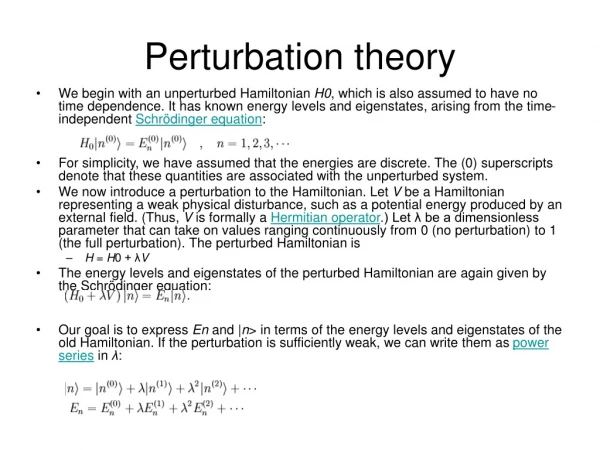
Perturbation theory. We begin with an unperturbed Hamiltonian H0 , which is also assumed to have no time dependence. It has known energy levels and eigenstates, arising from the time-independent Schrödinger equation :

E N D
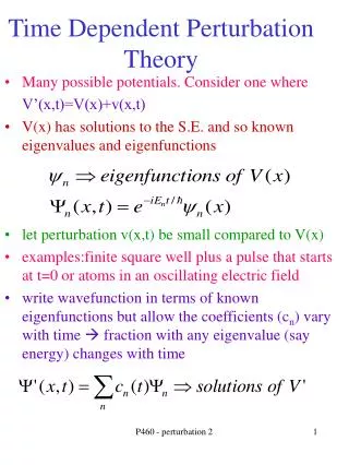
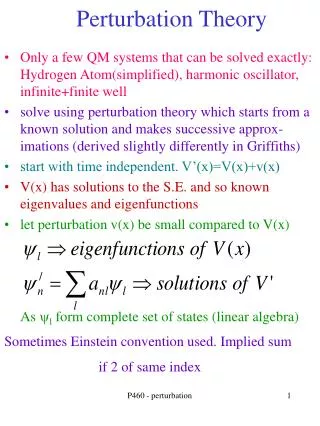
Perturbation theory • We begin with an unperturbed Hamiltonian H0, which is also assumed to have no time dependence. It has known energy levels and eigenstates, arising from the time-independent Schrödinger equation: • For simplicity, we have assumed that the energies are discrete. The (0) superscripts denote that these quantities are associated with the unperturbed system. • We now introduce a perturbation to the Hamiltonian. Let V be a Hamiltonian representing a weak physical disturbance, such as a potential energy produced by an external field. (Thus, V is formally a Hermitian operator.) Let λ be a dimensionless parameter that can take on values ranging continuously from 0 (no perturbation) to 1 (the full perturbation). The perturbed Hamiltonian is • H = H0 + λV • The energy levels and eigenstates of the perturbed Hamiltonian are again given by the Schrödinger equation: • Our goal is to express En and |n> in terms of the energy levels and eigenstates of the old Hamiltonian. If the perturbation is sufficiently weak, we can write them as power series in λ:
Plugging the power series into the Schrödinger equation, we obtain We will set all the λ to 1. Its just a way to keep track of the order of the correction • Expanding this equation and comparing coefficients of each power of λ results in an infinite series of simultaneous equations. The zeroth-order equation is simply the Schrödinger equation for the unperturbed system. The first-order equation is • Multiply through by <n(0)|. The first term on the left-hand side cancels with the first term on the right-hand side. (Recall, the unperturbed Hamiltonian is hermitian). This leads to the first-order energy shift: • This is simply the expectation value of the perturbation Hamiltonian while the system is in the unperturbed state. This result can be interpreted in the following way: suppose the perturbation is applied, but we keep the system in the quantum state |n(0)>, which is a valid quantum state though no longer an energy eigenstate. The perturbation causes the average energy of this state to increase by <n(0)|V|n(0)>. However, the true energy shift is slightly different, because the perturbed eigenstate is not exactly the same as |n(0)>. These further shifts are given by the second and higher order corrections to the energy.
En(1) En(2) We get • so the idea is, for any quantity to do an expansion like this • NOTE – it only works if the corrections are small and get smaller!