Download
1 / 23
330 likes | 724 Views
4.4 Linearization and Differentials. Linearization. Linearization uses the concept that when you zoom in to the graph at a point the y-values of the curve are very close to the y-values of the tangent line. (3, f(3). 3. Linearization. We can approximate

E N D
Linearization • Linearization uses the concept that when you zoom in to the graph at a point the y-values of the curve are very close to the y-values of the tangent line (3, f(3) 3
Linearization • We can approximate without a calculator by using the tangent line to f(x) at (3, f(3)) which is (3, f(3) 3
Linearization • We can approximate without a calculator by using the tangent line Approximate value Actual value
Linearization Note that the closer x is to 3 the better the approximation
is the standard linear approximation of f at a. To find the linearization of f(x) at the point (a, f(a)) Start with the point/slope equation: linearization of f at a The linearization is the equation of the tangent line, and you can use the old formulas if you like.
Example • Find the linearization L(x) of f(x) at x = a. • Compare f(a + 0.1) to L(a + 0.1)
Example • Find the linearization of at x = 0. Use it to approximate:
Example • Find the linearization of y = cosx at x = 0. Use it to approximate cos(0.5).
Example • Choose a linearization with center not at a but nearby so that the derivative will be easy to evaluate.
Example • Use linearization to find the value of at x = 0.12 to the nearest hundredth.
Differentials: When we first started to talk about derivatives, we said that becomes when the change in x and change in y become very small. dy can be considered a very small change in y. dx can be considered a very small change in x.
Let be a differentiable function. The differential is an independent variable. The differential is: dy is dependent on x and dx
Examples: a) Find dyb) Evaluate dy for the given values of x and dx • y = x2 – 4x ; x = 3, dx = 0.5 • y = xlnx; x = 1, dx = 0.1
Differentials can be used to estimate the change in y when x = a changes to x = a + dx True ChangeEstimated Change
Example: Consider a circle of radius 10. If the radius increases by 0.1, approximately how much will the area change? very small change in r very small change in A (approximate change in area)
(approximate change in area) Compare to actual change: New area: Old area:
Example • The earth’s radius is 3959 + 0.1 miles. What effect does a tolerance of + 0.1 miles have on the estimate of the earth’s surface area?
Example • Estimate the volume of material in a cylindrical shell with a height of 15m, radius 10m and shell thickness 0.2m.