Structural modelling: Causality, exogeneity and unit roots

1. Structural modelling: Causality, exogeneity and unit roots Andrew P. Blake CCBS/HKMA May 2004

2. What do we need to do with our data? • Estimate structural equations (i.e. understand what’s happening now) • Forecast (i.e. say something about what’s likely to happen in the future) • Conduct scenario analysis (i.e. perform simulations) to inform policy

3. What do we need to know? • Inter-relationships between variables • Causality in the Granger sense • Exogeneity • Concepts • Unit roots • Spurious regression • Role of pre-testing • Appropriate single equation methods

5. Inter-relationships between variables Period t Period t+1 xt xt+1 yt yt+1

6. How best to estimate an equation? • Single equation structural model (estimated by OLS) • Single equation reduced form (IV/OLS) • Structural system (estimated by TSLS, 3SLS or by a system method - SUR, FIML) • Unrestricted VAR (OLS) • VECM (FIML)

7. xt is autoregressive Period t Period t+1 xt xt+1 yt yt+1

8. xt has an autoregressive representation Period t Period t+1 xt xt+1 yt yt+1

9. xt has an ARMA representation } Structural system Reduced form

10. Granger Causality Period t Period t+1 xt xt+1 yt yt+1

11. Vector autoregressions (VARs) Period t Period t+1 xt xt+1 yt yt+1 Needs to be modelled to have a structural interpretation

12. Granger causality • If past values of y help to explain x, then y Granger causes x • Statistical concept • A lack of Granger causality does not imply no causal relationship

13. GC tested by an unrestricted VAR • Definition of Granger Causality: • y does not Granger cause x if a12=b12=...=0 • x does not Granger cause y if a21=b21=...=0 • NB. x and y could still affect each other in the same period or via unmeasured common shocks to the error terms.

14. Eviews Granger causalitytest result Null Hypothesis F-Statistic Probability x does not Granger Cause y F1 P1 y does not Granger Cause x F2 P2 • The closer P1 is to zero, the less the likelihood of accepting the null that x does not Granger cause y. • (P1<0.10 : at least 90% confident that s1 Granger causes s2). • P1 should be less than 0.10 for us to be reasonably confident that x Granger causes y.

15. Leading indicators y is a leading indicator of x if • y Granger causes x; • x does not Granger cause y; • and y is weakly exogenous.

17. Criticisms of Granger causality • Granger causality can be assessed using an unrestricted VAR - not tied to any particular theory • How would you explain to your governor when it goes wrong? • It depends on the choice of lags, data frequency and variables in VAR

18. Exogeneity • Engle et al. (1983) • Separate parameters into two groups • Those that matter, those that don’t • These are endogenous and weakly exogenous variables • In practice a bit more complicated than that

19. Exogeneity (cont.) • Correct assumptions of exogeneity simplify modeling, reduce computational expense and aid interpretation • But incorrect assumptions may lead to inefficient or inconsistent estimates and misleading forecasts

20. Exogeneity (cont.) • A variable is exogenous if it can be taken as given without losing information for the purpose at hand • This varies with the situation • We do not want the independent variables to be correlated with the regressors • If they are, the estimates will be biased

21. Relationships between variables Period t Period t+1 xt xt+1 yt yt+1 • We do not want the black arrows • We need to understand the red arrows

22. Both demand and supply shocks

23. OLS is unable to identify either the demand or supply curve

24. Only supply shocks

25. We can identify the demand schedule using OLS

26. Weak exogeneity • Is y weakly exogenous with respect to x? • Do values of current x affect current y? • Are x and y both affected by a common unmeasured third variable? • Does the range of possible values for the parameters in the process that determines x affect the possible values of those that determine y

27. Weak exogeneity: example 1 • Money demand function: • Would you estimate this as a single equation using OLS? • Very unlikely that money does not affect real output or the nominal interest rate

28. Weak exogeneity: example 2 • Uncovered interest parity: • Tests of UIP have performed very poorly, but ... • No risk premia and monetary policy might react to exchange rate changes

29. Interest rate differentials Exchange rate change Question: how would you test for exogeneity in UIP?

30. Weak exogeneity: example 3 • In UK consumption had been forecast using single-equation ECM • But relationship broke down in late 1980s • Problem was that possibility that wealth reactions to disequilibrium had been ignored

31. Single Equation ECM Dynamic terms Long run

32. Vector ECMS Halfway between structural VARs and unrestricted VARs

33. Strong exogeneity • Necessary for forecasting • Is y strongly exogenous to x? • Is y weakly exogenous to x • Does x Granger cause y? • Need the answers to be yes and no respectively

34. Strong exogeneity: example • First order VAR, ‘core’ and non-‘core’ inflation: • Given a forecast of {yt} can we forecast {xt}? • If y is not strongly exogenous to x, feedback problems

35. Super exogeneity • Necessary for policy/scenario analysis. Is y super exogenous to x? • Is y weakly exogenous to x? • Is the relationship between x and y invariant? • Need the answers to be yes to both

36. Invariance • The process driving a variable does not change in the face of shocks • Linked to ‘deep parameters’ • Example: the Lucas critique

37. Testing for weak exogeneity: orthogonality test • Estimate a reduced form (marginal model) for x, regress x on any exogenous variables of the system • Take residuals from this reduced form and put them into the structural equation for y • If they are significant then x is not weakly exogenous with respect to the estimation of c10

38. Testing for weak exogeneity with respect to c(lr) • Estimate a reduced form (marginal model) for x: regress x on exogenous variables of system, including lagged ECM term involving x and y • Test if coefficient of ECM term is significant • If it is, then x is not weakly exogenous with respect to the estimation of long-run coeff, c(lr) • Consequence is that estimate is inefficient

39. Stationarity • Why should we test whether series are stationary? • A non-stationary time series implies that shocks never die out • The mean, variance and higher moments depend on time • Standard statistics do not have standard distributions • Problem of spurious regression

40. Non-stationarity • Start with the following expression yt= +yt-1 + utu, 2 • Substitute recursively: yt=  n + nyt-n + n-1jut-j • The variable will be non-stationary if = E(y)=t Var(y) = Var(n-1ut-j - t) = t2 • Displays time dependency

41. Non-stationarity (cont.) • t is a stochastic trend • The series drifts upwards or downwards depending on sign of ; increases if positive • Stationary series tend to return to its mean value and fluctuate around it within a more-or-less constant range • Non-stationary series has a different mean at different points in time and its variance increases with the sample size

42. Non-stationarity (cont.) • Mean and variance increase with time • yt=  n + nyt-n +n-1jut-j • If = then shocks never die out • If |  |<1 as n, then y is like a finite MA • What do non-stationary series look like? • Could show made-up series (with and without drift)

43. Difference vs trend stationarity • Compare previous equation with yt = a + b t + ut E(y) = a + b t var(y) = 2 • bt - deterministic trend • But stationary around a trend E(y - b t) = a

44. Difference vs trend stationarity (2) • Compare two generated series • Stationary around trend • Difference stationary are non-constant around a trend • But can be difficult to tell apart • Also difficult to tell series with AR coefficients 1 and 0.95

45. Difference vs trend stationary

46. Difference vs trend stationarity • Can you tell the difference? xt= 1 + xt-1 + 0.6 ut zt = 1 + 0.15 t + 0.8 et • Can you tell the difference with a near-unit root?

47. Unit root vs near-unit root

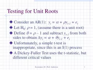
48. Testing for unit roots • Dickey-Fuller test • Write yt= yt-1 + et as yt - yt-1= (-1)yt-1 + et Null: Coefficient on lagged value 0, vs < 0

49. Dickey-Fuller tests • Test akin to t-test but distributions not standard • Depends if series contains constant and/or trends • Must incorporate this into DF test • Augmented DF test - use lags of dependent variable to remove serial correlation • All of these must be checked against relevant DF statistic • But introducing extra variables reduces power

50. Unit versus near-unit roots • Thus difficult to tell the difference between two series over small samples • Low power of ADF tests (sample of 400) x: ADF statistic -0.77048 p-value 0.8258 w: ADF statistic -6.90130 p-value 0.0000 • Small sample (40 observations) x: ADF statistic 0.39323 p-value 0.9804 w: ADF statistic -0.49216 p-value 0.8828