Computer Graphics SS 2014 Ray-Tracing Acceleration

1. Computer Graphics SS 2014 Ray-Tracing Acceleration Rüdiger Westermann Lehrstuhl für Computer Graphik und Visualisierung

2. Ray tracingacceleration • Acceleration techniques for ray tracing • Keep in mind that the complexity of ray tracing is O(m x p),where m is the number of pixels and p is the number of objects in the scene • For each ray we have to check for intersections with every object • If we have polygonal objects and the entire scene consists of n polygons, the complexity is O(m x n) • For each ray we have to check for intersections with every polygon of every object

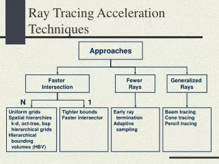
3. Ray tracingacceleration • Classification of acceleration techniques for ray tracing • Faster ray-object intersections • Efficient intersectors • Fewer ray-object intersections • Bounding volumes (boxes, spheres) • Space subdivision • Fewer rays • Adaptive tree-depth control • Stochastic sampling

4. Ray tracingacceleration • Faster ray-object intersections • A Fast Triangle-Triangle Intersection Test (1997)  Tomas Möller: Journal of Graphics Tools • Intersectionpoint R(t)=o + tDinbarycentriccoordinatesu,v: (1-u-v)V0+uV1+vV2 =o+tD-tD+ uV1-uV0+vV2-vV0 = o-V0[-D,V1-V0, V2-V0][t,u,v]T = o-V0

5. Ray tracingacceleration • Ray-triangleintersection • Solvingthesystemofequations (Cramers rule)

6. Ray tracingacceleration • Fewer ray-object intersections • Bounding volumes (boxes, spheres) • A boundingvolumeis a simple volumedescriptionthatisguaranteedtocontain a morecomplexobject, e.g. a sphere/box thatcovers a polygonal model • Test rayagainstboundingvolumefirst, and onlyifitintersectsthisvolumetherayistestedagainstthepolygons

7. Ray tracingacceleration • Fewer ray-object intersections • Bounding volumes (boxes, spheres) • Increase time tocomputeintersections, but reduce time whenraymissestheboundingvolume • Providebound on intervalofintersection

8. Ray tracingacceleration • Fewer ray-object intersections • Bounding volumes (boxes, spheres) • With simple bounding volumes, ray casting still requires O(p) intersection tests • Idea: use tree data structure • Larger bounding volumes contain smaller ones etc. • Often reduces complexity to O(log(p))

9. Ray tracingacceleration • Fewer ray-object intersections using hierarchical bounding volumes • Ray intersection algorithm recursively descends tree • If ray misses bounding volume, no intersection • If ray intersects bounding volume, recurse with enclosed volumes and objects • Maintain near and far bounds to prune further • Overall effectiveness depends on model and constructed hierarchy

10. Ray tracingacceleration • Bounding volumes • Classesofboundingvolumes • BoundingSpheres • Axis-alignedBounding Boxes = AABB • OrientedBounding Boxes = OBB

11. Ray tracingacceleration • Boundingvolumes - properties Decreasingcost(intersectionwith BV + BV construction) Increasingcomplexity, but bettertightnessof fit

12. Ray tracingacceleration • Boundingspheres • Construction: • Determinedby maximal distancebetweenanyobjectsvertexand thecenterof all vertices • Computebounding box and centersphereat box center • Large regionwasted in general • Analyticdescription • Allows for fast conservative check • Hierarchybyincreasinglysmaller (top-down) / larger (bottom-up) spheres

13. Ray tracingacceleration • Boundingsphereshierarchy

14. Ray tracingacceleration • Axis alignedboundingboxes • Hierarchybysuccessivesplitsalongx/y/z-axis • Possiblerefinementcriteria: • Longestaxis • Numberofelements in each BV • Size ofboundingvolumes

15. Ray tracingacceleration • OrientedBounding Boxes (OBB) • Proposedby Gottschalk in 1996 AABBsOOBBs

16. Ray tracingacceleration • OrientedBounding Boxes (OBB) • Complexconstructionof OBB in a pre-process • Tobediscussed in thecourseImage Synthesis (WS12/13) • Fix in objectcoordinatesystem • Goodadaptiontoobjectgeometry • Nochangeof OBBs duringobjectmovements! • Efficientintersectiontestbetweenrayandvolume

17. Ray tracingacceleration • Spatialsubdivision • A divisionofspaceintodisjoint sub-regions, i.e. a partition • For each region, stores a list of objects/polygons contained in this region • At run-time, only test sub-regions that are hit • General problem of all spatial subdivision schemes: objects/polygons might get cut by region boundaries • Solution: either store objects/polygons in all regions they overlap, or cut into halves – increases number of polygons that have to be stored

18. Ray tracingacceleration • Spatialsubdivision – problems • Needs tostore 5 insteadof 2 references • Per subregion: testagainst all (also exterior) objectparts subregion1 subregion2 objectList: C1, C2 C2 partition1: C1 C2 C1 partition2: C1 C1 partition3: C1 partition4: subregion3 subregion4

19. Ray tracingacceleration • Spatialsubdivision – problems • Needs tostore 3 objectsinsteadof 1 objectList: C1 // onelinesegment // C1 isclippedatsubregionboundaries subregion1 subregion2  objectList: C1.1, C1.2, C1.3 C1.1 C1.2 partition1: C1.1 partition2: C1.2 C1.3 partition3: partition4: C1.3 subregion3 subregion4

20. Ray tracingacceleration • Uniform spatialsubdivision - grids • A 3D array of cells, a regular space partition • Rays step from cell to cell and test against the objects/polygons in each cell

21. Ray tracingacceleration • Properties of regular grids • Grid traversal, i.e. from cell to cell, is very fast • Poor choice when geometry is clustered locally, i.e. many cells do not contain any polygon • Keep in mind that a grid needs to store all cells regardless of whether they contain something or not • Resolution of grid • Too low: too many polygons per cell • Too high: too many empty cells to traverse and store • Non-uniform spatial subdivision is more flexible • Can adjust to geometry “density”

22. Ray tracingacceleration octree kd-tree bsp-tree • A kd-treeis a specializationof a bsp-tree, wherethepartitioning planes areaxis-aligned, canmovearbitrarily, andsplitsoccur in a fixedorder, e.g., x – y – z. • In an octree, thepartitioning planes areaxis-aligned, always half thespace, andsplitsoccursimultaneouslyalong x/y/z.

23. Ray tracingacceleration • Adaptive subdivision - octrees/quadtrees • Recursiveregularsubdivisionofspaceinto 8/4 subspaces • Onenodeissplitinto 8/4 childnodes • Adaptivelysubdividethe 8/4 children • 3/2 cases (splitting planes) havetobeconsidered 1 2 y 3 4 x Quadtree 1 2 3 4 1 2 3 4

24. Ray tracingacceleration • Adaptive subdivision - octrees/quadtrees

25. Ray tracingacceleration • Adaptive subdivision - Binary Space Partitioning • Generalizationofbinarysearchtreesfor dim> 1 • Searchcomplexityfor a singleobjectiswithin O(1) toO(log n) (withnbeingthenumberofobjects) • Recursivespacepartitioningbymeansofarbitrarilypositionedpartitioningplanes

26. Ray tracingacceleration P1 • Adaptive subdivision - Binary Space Partitioning • Subdivision and thecorresponding BSP-tree P2 P3 A C B D A B P2 Eachnodecorrespondsto a partitioning plane Leafnodesstorelinksto objects/polygons D P3 C P1

27. Ray tracingacceleration P1 • Bsp-treescaneffectivelyreducethenumberofray-polygon intersections • In thiscaseonly traversenode P1 and P3 P2 P3 A C B D A B P2 D P3 C P1

28. C A B D Ray tracingacceleration P1 • Bsp-treesareeffective in determiningthevisibility orderofobjects • Sort objects so that an object can never occlude any object in the sorted sequence before • Recurseintothepartitonfirstthatcontainstheviewer P2 P3 A C B D A B P2 D P3 C P1

29. Ray tracingacceleration • Bsp-treeconstruction 1)Generate candidate split-plane locations 2)Evaluate cost function C at each location 3)Pick the one with the lowest cost

30. Ray tracingacceleration • Bsp-tree (kd-Tree) construction • Thereareinfinitelymanycandidate planes • Chose candidate planes thatarealignedwiththefacesofobjectboundingboxes

31. Ray tracingacceleration • The cost function C • It should measure the work that has to be done if a certain plane is selected • The plane subdivides space into the “left” and “right” half-spaces • The work of one ray intersecting the left/right half-space is proportional to the number of objects in the left/right half-space • Question: of all rays intersecting the entire space, how many intersect the left/right half-space

32. Ray tracingacceleration • The number of rays in a given direction that hit an object is proportional to its projected area • Crofton’s Theorem statesthat Ā=S/4, where Ā is the average projected area in all directions and S is the surface area (convex surfaces)

33. Ray tracingacceleration • The probability of a ray r hitting a convex shape that is completely inside a convex cell equals Si := surfaceareaofi-thobject

34. Ray tracingacceleration • Assuming intersection time ti and traversal time tt, number of objects in a and b is Na and Nb, and then (Surface Area Heuristic) b a

35. Ray tracingacceleration • bsp-treeconstructionusesfacesoftriangle-AABBs aspartitioning planes