Download
1 / 59
700 likes | 1.03k Views
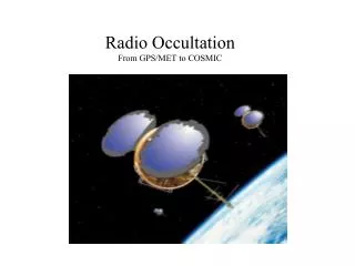
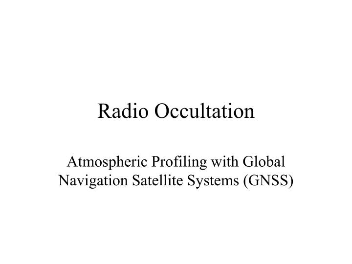
Radio Occultation. Atmospheric Profiling with Global Navigation Satellite Systems (GNSS). Overview. The Idea: A first look at planetary atmospheres Next step: Applying the technique to Earth The principles The GPS system and the GPS measurement How RO works

E N D
Radio Occultation Atmospheric Profiling with Global Navigation Satellite Systems (GNSS)
Overview • The Idea: A first look at planetary atmospheres • Next step: Applying the technique to Earth • The principles • The GPS system and the GPS measurement • How RO works • Unique characteristics of the observations • Satellite missions • Science Applications • Meteorology • Climate • Space Weather
Question: How can we learn if planets have an atmosphere? Send a space probe from Earth to the far side of the planet in question and send a known radio frequency back to Earth. As the signal grazes the planet’s Limb it’s radio signal is occulted (thus radio occultation) If the planet has no atmosphere the radio signal received on Earth will travel on a straight line …. but if there is an atmosphere the ray will be bent!
Question: But how do we know if the ray is bent? For a straight ray the Doppler shift is caused only by the relative motion of the transmitter relative to the receiver - and can be predicted based on orbital mechanics For a bent signal the Doppler shift will noticeably different than predicted based on orbital mechanics only! Measure the Doppler frequency shift of the received radio signal on Earth.
Planetary Radio Occultation Mariner IV at Mars July 1965 Radio occultation was first applied to Planetary atmospheres by teams at Stanford U. and NASA/JPL
Mariner V at Venus 19 October 1967 Subsequently RO was used to study the atmospheres of many planets
Low-Earth Orbiter LEO Transmitter The signal is received on the LEO And atmospheric properties can be obtained The same measurement principle can also be used to observe Earth’s atmosphere
There are some key advantages for radio occultation on Earth
Signals Abundant GPS Glonass Galileo --------------- 60–90 sources in space
~3000 km GPS Signal Coverage Two L-band frequencies: L1: 1.58 GHz L2: 1.23 GHz
The GPS Signal Spectrum Carrier Carrier + Code
A GPS receiver in LEO can track GPS radio signals that are refracted in the atmosphere GPS Satellite LEO Orbit Atmosphere Radio Signal LEO Satellite
Occultation Geometry • During an GPS occultation a LEO ‘sees’ the GPS rise or set behind Earth limb while the signal slices through the atmosphere Occultation geometry • The GPS receiver on the LEO observes the change in the delay of the signal path between the GPS SV and LEO • This change in the delay includes the effect of the atmosphere which delays and bends the signal
Bending angle Earth Transmitted wave fronts Wave vector of received wave fronts From orbit determination we know the location of source and We know the receiver orbit Thus we also know Determining Bending from observed Doppler (a) We measure the Doppler frequency shift: And compute the bending angle
a vT Deriving Bending Angles from Doppler • The projections of satellite orbital motion of transmitter and receiver along the ray path produces a Doppler frequency shift • After correction for clock and relativistic effects, the Doppler shift, fd, of the transmitter frequency, fT, is given as • where: c is the speed of light and the other variables are defined in the figure with VTr and VTq representing the radial and azimuthal components of the transmitting spacecraft velocity. From Doppler + orbits we obtain bending as a function of impact parameter
Define the refractional radius x=nr, where n=1+N*10-6 Now we have a profile of refractivity as a function of “x” We compute the “mean sea level height” of the observation: hmsl=x-Rc-G (where Rc is radius of curvature, and G is the geoid height)
Definition of Altitude in Radio Occultation Steps taken in determining “MSL” altitude z • Determine the lat/lon of the ray path perigee at the‘occultation point’ (that point where the excess phase exceeds 500 meters) • Compute the center of sphericity (C) and radius of curvature (Rc) of the intersection of the occultation plane and the reference ellipsoid at the assigned lat/lon. • Do the Abel inversion in the reference frame defined by the occultation plane and C. • Now height r is defined as the distance from the perigee point of the ray path to C. • G is the geoid correction. We currently use the JGM2 geoid. The geometric height in the atmosphere is computed : z = r - Rc - G G - geoid height z - geometric height r reference ellipsoid Rc - radius of local curvature of ref. ellipsoid Center of curvature C
Atmospheric refractivity N=(n-1)*10-6 Ionospheric term dominates above 70 km Hydrostatic (dry) wet terms dominates at lower altitudes Wet term becomes important in troposphere (> 240 k) and Can be 30% of refractivity in tropics Liquid water and other aerosols are generally ignored
Observed Atmospheric Volume L~300 km Z~1 km
Unique Attractions of GPS Radio Occultation 1. High accuracy: Averaged profiles to < 0.1 K 2. Assured long-term stability 3. All-weather operation 4. Global 3D coverage: stratopause to surface 5. Vertical resolution: ~100 m in lower trop 6. Independent height & pressure/temp data 7. Compact, low-power, low-cost sensor
CHAMP Sunsat IOX Ørsted RO Missions SAC-C GPS/MET GRACE
GPS/MET Proof of Concept Mission The first RO profile from Earth
The next wave… COSMIC/FormoSat3 (6) EQUARS C/NOFS METOP
Constellation Observing System for Meteorology Ionosphere and Climate (ROCSAT-3) • 6 Satellites launched in 2006 • Orbits: alt=800km, Inc=72deg, ecc=0 • Weather + Space Weather data • Global observations of: • Pressure, Temperature, Humidity • Refractivity • TEC, Ionospheric Electron Density • Ionospheric Scintillation • Demonstrate quasi-operational GPS limb sounding with global coverage in near-real time • Climate Monitoring • Geodetic Research COSMIC at a Glance
Location of Profiles 1.5 months after launch Final constellation
GPS Occultation receiver Mission science payloads • High-resolution (1 Hz) absolute total electron content (TEC) to all GPS satellites in view at all times (useful for global ionospheric tomography and assimilation into space weather models) • Occultation TEC and derived electron density profiles (1 Hz below the satellite altitude and 50 Hz below ~140 km), in-situ electron density • Scintillation parameters for the GPS transmitter–LEO receiver links • Data products available within 15 - 120 minutes of on-orbit collection • Tiny Ionosphere Photometer (TIP) • Nadir intensity on the night-side (along the sub-satellite track) from radiative recombination emission at 1356 Å • Derived F layer peak density • Location and intensity of ionospheric anomalies (Auroral Oval) • Tri-band Beacon (TBB) • Phase and amplitude of radio signals at 150, 400, and 1067 MHz transmitted from the COSMIC satellites and received by chains of ground receivers. • TEC between transmitter and receivers • Scintillation parameters for LEO transmitter - receiver links
COSMIC + EQUARS Soundings in 1 Day Occultation locations for COSMIC (6 s/c, 3 planes) and EQUARS, 24 hrs COSMIC EQUARS Radiosondes
Science Applications Weather Climate Space Weather
Evolution of forecast skill for northern and southern hemispheres Courtesy, Simmons 2004 Evolution of forecast skill for the northern and southern hemispheres: 1980-2001. Anomaly correlation coefficients of 3, 5, and 7-day ECMWF 500-mb height forecasts for the extratropical northern and southern hemispheres, plotted in the form of running means for the period of January 1980-August 2001. Shading shows differences in scores between hemispheres at the forecast ranges indicated (from Holingsworth, et al. 2002).
The GPS-MET Experiment on MicroLab-I 1995 - ?
RO provides best results between 8-30 km (effects of moisture and ionosphere are negligible). Is capable of resolving the structure of the tropopause and gravity waves above the tropopause. “dry temperature” computed from refractivity assuming no water vapor Figure from the paper by Nishida et al., J. Met. Soc. Japan, 78(6), p.693, 2000.
Case 1: Hurricane Isabel (2003) A Equivalent potential temperature • Developed in the lower Atlantic ocean, tracked northwest and landed at North Carolina coast on Sept 18, 2003 • The hurricane was category 4 or 5 for a period of 6 days. • The WRF simulation covered a period when the hurricane was category 2. • 24-h forecast from 4-km WRF simulation, valid at 0000 UTC 17 September 2003. B Radar reflectivity B A
CHAMP-SACC Profile Comparison Full Profiles Avg Delta Profiles Height, km Height, km Temp, K D Temp, K Hajj et al., 2004
GPS RO Data Impact on Weather Prediction From Healey et al. GRL, 2004
Effects of CO2 increase on climate change simulated by NCAR Climate System Model (CSM)
Global Temperatures from 1995- 2005 50 mb and 100 mb levels
Polar temperatures at 50 mb from 1995-2005 North Pole South Pole