Download
1 / 18
190 likes | 520 Views
Speech Coding. Nicola Orio Dipartimento di Ingegneria dell’Informazione. IV Scuola estiva AISV, 8-12 settembre 2008. Speech Compression. Handling speech with other media information such as text, images, video, and data is the essential part of multimedia applications

E N D
Speech Coding Nicola Orio Dipartimento di Ingegneria dell’Informazione IV Scuola estiva AISV, 8-12 settembre 2008
Speech Compression • Handling speech with other media information such as text, images, video, and data is the essential part of multimedia applications • The ideal speech coder has a low bit-rate, high perceived quality, low signal delay, and low complexity. • Delay • Less than 150 ms one-way end-to-end delay for a conversation • Processing (coding) delay, network delay • Over Internet, ISDN, PSTN, ATM, … • Complexity • Computational complexity of speech coders depends on algorithms • Contributes to achievable bit-rate and processing delay
Speech coding • Standard voice channel: • analog: 4 kHz slot (~ 40 dB SNR) • digital: 64 Kbps = 8 bit µ-law x 8 kHz • How to compress? • Exploit redundancy • signal assumed to be a single voice, not any waveform • Code only what is needed • intelligibility • speaker identification • Source-filter decomposition • vocal tract shape & fundamental frequency change slowly
Taxonomy of Speech Coders Speech Coders Waveform Coders Source Coders Time Domain: PCM, ADPCM Frequency Domain: e.g. Sub-band coder, Adaptive transform coder Linear Predictive Coder Vocoder
The ancestor: Channel Vocoder (1940s-1960s) • Source-filter decomposition • filterbank breaks into spectral bands • transmit slowly-changing energy in each band • 10-20 bands, perceptually spaced • Downsampling • Excitation with a pitch / noise model
LPC encoding • The classic source-filter model • Compression gains: • filter parameters are ~slowly changing • excitation can be represented many ways
Model speech production system as an auto-regressive model: Model parameters are computed for speech segment (~30 ms). Parameters {a(k); k=1:p} are found by solving a Toeplitz system of equations. Transfer function To encode speech, one may transmit the quantized parameters {a(k)} and G or equivalent parameter set. The model order is 8-10 in most speech coding standards. unvoiced G v/u voiced N random sequence generator u[n] periodic pulse train generator Vocal Tract Model H(z) = 1 1akz-k P k = 1 Linear Predictive Code
LPC Speech Coder LPC filter Synthesizer Voice/ Un-voice Channel Encoder Buffer Decoder Pitch Analysis Excitation
Encoding LPC filter parameters • For ‘communications quality’: • 8 kHz sampling (4 kHz bandwidth) • ~10th order LPC (up to 5 pole pairs) • update every 20-30 ms → 300 - 500 param/s • Representation & quantization • {ai} - poor distribution,can’t interpolate • reflection coefficients {ki}:guaranteed stable • log area ratios (LAR) - stable • Bit allocation (filter): • GSM (13 kbps):8 LARs x 3-6 bits / 20 ms = 1.8 Kbps
Excitation • Excitation as LPC residual is already better than raw signal: • save several bits/sample, still > 32 Kbps • Crude model: U/V flag + pitch period • ~ 7 bits / 5 ms = 1.4 Kbps → LPC10 @ 2.4 Kbps
CELP • Code excited linear predictive (CELP) speech coding. • White noise input does not give satisfactory results: • the residue sequence still contains important information for speech synthesis • it is necessary to send the residue to receiving end too. • To save space, use vector quantization (VQ) technique to encode the residue sequence • Hence the name “code excited”. • In CELP, each code book is a linear vector containing 0 or 1 • each code word length is 60 samples • successive code words are overlapped by 58 samples • a linear search is performed to find the best code words as input to the LPC model.
CELP • Represent excitation with codebooke.g. 512 sparse excitation vectors • linear search for minimum weighted error?
GSM Speech Encoder Regular pulse excitation (RPE) Pre-processing STP LTP Order = 8 LAR coefficients Hamming Window Short Term Prediction MUX Long Term Prediction Gain, pitch Segmentation LPC Inverse Filter 20ms Grid Selection + LPF Pre-emphasis Speech input
GSM Decoding De-Mux RPE Decoding LTP Synthesis STP Synthesis Post- Processing Pitch, gain LAR Coefficients
Tasks: LPC analysis filter to calculate the coefficients Long term prediction for pitch analysis need to find delay D and gain VQ search during CELP encoding – Most time consuming FIR filtering for pre- and post processing Often implemented in DSP chips for embedded applications (e.g. cell phone). The parameter quantization part needs bit-level operation. Implementation Issues
Vector Quantization: Definition • Blocks: form vectors • A sequence of audio • A block of image pixels • A vector quantizer maps k-dimensional vectors in the vector space R k into a finite set of vectors • Unquantized vector: • Quantized vector: • Reconstruction vector (codeword): • Codebook: the set of all the codewords: • Voronoi region: nearest neighbor region