Download
1 / 49
530 likes | 921 Views
Introduction to Labor Supply. Labor supply facts Men: labor force participation rates declined from 80% in 1900 to 70% in 2012. Women: labor force participation rates rose from 21% in 1900 to 57.7% in 2012. Average hours worked fell from 40 to 34 per week during the same time period.

E N D
Introduction to Labor Supply Labor supply facts Men: labor force participation rates declined from 80% in 1900 to 70% in 2012. Women: labor force participation rates rose from 21% in 1900 to 57.7% in 2012. Average hours worked fell from 40 to 34 per week during the same time period.
LOTTERY WINNINGS AND LABOR SUPPLY • What is the elasticity of labor supply with respect to a change in non-labor income? • This paper identifies an exogenous variation in non-labor income by exploiting the random assignment of large amounts of money to major-prize winners of the Megabucks lottery in Massachusetts during the period 1984 to 1988. • The key assumption underlying the analysis is that the size of the lottery prize is random across all individuals (“winners” and “non-winners”) in the sample.
LOTTERY WINNINGS AND LABOR SUPPLY • 496 Survey Participants • 237 “Winners” (20 year payout, mean = $55K/yr) • 43 “Big Winners” (20 year payout, > $100K/yr) • 259 “Non-winners” (one payout < $5000) • Data were collected on demographic, financial, and socio-economic background variables and from the SSA on six years of pre- and post-lottery earnings data
LOTTERY WINNINGS AND LABOR SUPPLY • The marginal propensity to earn labor income (MPE), consume, and save out of additional non-labor income was calculated for all respondents, “non-winners”, “winners”, and “big winners” • A difference-in-differences estimate of the MPE is calculated as the ratio of the difference in the average change in earnings for the “winners” and “non-winners” and the difference in the value of the average prize for the same two groups
LOTTERY WINNINGS AND LABOR SUPPLY • “Winners”: ∆Y = –$1,877 • “Non-winners”: ∆Y = $448 • MPE = (-$1877 – $448)/($55,000 – $0) = -0.042 (0.016) • A $10,000 increase in the annual payout from the lottery winnings reduces annual earnings by 4.2% or $420 • “Big winners”: MPE = -0.059 (0.018)
LOTTERY WINNINGS AND LABOR SUPPLY • Regression-based approach: • Y = + X + V + V2 + • Y is average post-lottery earnings • X is a set of control variables (age, education, sex, etc.) • V is the annual lottery payout • is a random error term
LOTTERY WINNINGS AND LABOR SUPPLY • Hypotheses: • ∆Y/∆V = + 2V < 0 (leisure is a normal good) • < 0 (MPE decreases as payout increases) • Results: • Typical estimate of the MPE is -0.11, evaluated at V = $32,000 • MPC for cars = 0.009 (0.002) • MPC for housing = 0.04 (0.01) • MPS = 0.158 (0.056) and increases with the amount of the prize payout
Current Population Survey (CPS) Labor Force = Employed + Unemployed LF = E + U Size of LF does not tell us about “intensity” of work. Labor Force Participation Rate LFPR = LF/P P = civilian population 16 years or older not in institutions. Measuring the Labor Force
Measuring the Labor Force Current population survey (CPS) Employment: Population Ratio (percent of population that is employed). EPR = E/P Unemployment Rate UR = U/LF
Labor force measurement relies on subjective interpretation of survey responses and likely understates the effects of a recession. Hidden unemployed: persons who have given up in their search for work and have therefore left the labor force. The employment rate (E/P) may be a better measure of fluctuations in labor-market activity than the labor-force participation rate or the unemployment rate. Measuring the Labor Force
Labor Force Participation Facts Labor force participation rate (LFPR) is greatest for all demographic groups between the ages of 25 and 55. LFPR increases with education. LFPR has decreased for men over the age of 65 from 63% in 1900 to under 23% in 2011.
More women than men work part-time. More men who are high school drop outs work than women who are high school drop outs. White men have higher participation rates and hours of work than black men. Labor Force Participation Facts
Average weekly hours of work of production workers, 1900-2010
Neo-Classical Model ofLabor-Leisure Choice Utility Function Measures satisfaction individuals receive from consumption of goods (G) and leisure (L). U = f(G, L) U is an ordinal (rank-order-preserving) index. The higher is U, the happier is the person.
Indifference Curves Downward-sloping, indicating the tradeoff between consumption of goods and consumption of leisure Higher indifference curves = higher utility Do not intersect Convex to the origin, indicating that opportunity costs increase or, alternatively, that preferences are “diverse”
Indifference Curves Goods ($) 500 450 400 40,000 Utils 25,000 Utils 100 125 150 Leisure (Hours)
Differences in Preferences Workers with steeper indifference curves value their leisure relatively more than workers with flatter indifference curves. Goods($) Goods($) U1 U1 U0 U0 Leisure (Hours) Leisure (Hours)
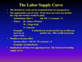
The Budget Constraint The budget constraint defines the worker’s opportunity set, indicating all of the consumption – leisure combinations the worker can afford. G = wh + V Goods consumption equals labor earnings (wages × hours of work) plus non-labor income (V). Since h = T – L, we can rewrite the budget constraint as G = w(T – L) + V.
Graphing the Budget Constraint Goods($) wT+V Budget Line E V Leisure (Hours) 0 T
Hours of Work Individuals choose goods and leisure to maximize utility. Optimal consumption is given by the point where the budget line is tangent to the indifference curve. At this point the marginal rate of substitution (MRS) between goods and leisure equals the wage. Any other goods– leisure bundle on the budget constraint would give the individual less utility.
Optimal Consumption and Leisure $1200 Y A $1100 P $500 U1 U* E $100 U0 Hours of Leisure 0 70 110 Hours of Work 0 110 40
The Effect of a Change in Nonlabor Income on Hours of Work Goods($) F1 F0 P1 U1 P0 $200 E1 U0 $100 E0 110 70 80 Leisure (Hours) An increase in nonlabor income leads to a parallel, upward shift in the budget line, moving the worker from point P0 to point P1. If leisure is a normal good, hours of work fall.
The Effect of a Change in NonlaborIncome on Hours of Work Goods ($) F1 P1 F0 U1 P0 $200 E1 U0 $100 E0 110 70 60 An increase in nonlabor income leads to a parallel, upward shift in the budget line, moving the worker from point P0 to point P1. If leisure is inferior, hours of work increase.
Backward-bending Labor Supply When the income effect dominates the substitution effect, the worker increases (decreases) hours of leisure (work) in response to a wage increase Goods ($) G U1 R D Q U0 D F P V E Leisure (Hours) 110 0 70 75 85
When the substitution effect dominates the income effect, the worker decreases (increases) hours of leisure (work) in response to a wage increase Upward-sloping Labor Supply Goods ($) U1 G R D Q U0 D F P V E 110 0 65 80 Leisure (Hours) 70
To Work or Not to Work? Is the market wage rate sufficiently attractive to “bribe” an individual to enter the labor force? Reservation wage: the wage rate at which the individual is indifferent between working and not working. Rule 1: if the market wage is less than the reservation wage, then the person will not work. Rule 2: the reservation wage increases as non-labor income increases
The Reservation Wage Goods ($) H Slope = -w Y G X UH E U0 Slope = -wr T 0 Leisure (Hours)
Reservation Wage and Labor Supply What is the relationship between hours worked and the wage rate at the “margin of indifference,” where w = wr? In response to a marginal increase in the wage rate, evaluated at h = 0 (L = T), there is only a substitution effect At wage rates slightly above the reservation wage, the labor supply curve is positively sloped (the substitution effect dominates the income effect).
The Backward Bending Labor Supply Curve Wage Rate ($) 25 20 10 Hours of Work 0 40 20 30
Labor Supply Elasticity The labor supply elasticity (hw) measures the responsiveness of hours worked to changes in the wage rate. hw= Percent change in hours worked divided by the percent change in wage rate. Labor supply elasticity less than 1 is wage-inelastic since hours of work respond proportionally less than the change in wages. Labor supply elasticity greater than 1 is wage-elastic since hours of work respond proportionally more than the change in wages.
Labor Supply of Women Substantial cross-country differences in women’s labor force participation rates Over time, female labor force participation rates have increased In most studies of female labor supply, the substitution effect dominates the income effect, implying an upward sloping labor supply curve
Source: Jacob Mincer, “Intercountry Comparisons of Labor Force Trends and of Related Developments: An Overview,”Journal of Labor Economics 3 (January 1985, Part 2): S2, S6. Growth in Female Labor Force Participation and the Wage Across Countries, 1960-1980
Policy Application: Welfare Programs and Work Incentives Cash subsidies reduce labor supply (income effect) Most welfare programs reduce labor supply (income effect and substitution effect) Most welfare programs reduce labor supply by increasing non-labor income, which raises the reservation wage, and imposing an implicit tax on wages, which reduces the net-of-tax wage rate
Effect of a Cash Subsidy on Labor Supply A take-it-or-leave-it cash subsidy of $500 per week moves the worker from point P to point G, and encourages the worker to leave the labor force. Goods ($) F G U1 500 U0 Leisure (Hours) 70 0 110 P
Effect of a Welfare Program on Labor Supply Goods ($) U0 U1 F slope = -$10 H D slope = -$5 Q R P $500 G D E Leisure (Hours) 0 100 70 110
The Earned-Income Tax Credit:Labor-Supply Effects The EITC increases the labor force participation rate of recipients in the targeted groups Eligibility for the EITC encourages some non-workers to start working, but never encourages a current worker to stop working The EITC produces an income effect for most recipients Hours worked among workers will decrease
The Earned-Income Tax Credit: 2012 Goods ($) F G Net wage is 21.06% below the actual wage 41,952 H 22,326 Net wage equals the actual wage J 18,326 17,090 Net wage is 40% above the actual wage 13,090 E Leisure (Hours) 110
Labor Supply over the Life Cycle Wage rates change over the worker’s lifetime Wages are low when young Wages rise with time and peak around age 50 Wages decline or remain stable after age 50 The changes in wage rates over the life cycle are “evolutionary” wage changes that alter the relative “price” (or opportunity cost) of leisure.
Evolutionary Wage-Rate Changes A person will work more hours when wages are relatively higher (i.e., the inter-temporal substitution effect dominates the income effect) The profile of hours of work over the life cycle will have the same shape as the age-earnings profile. Inter-temporal substitution hypothesis: people substitute between work and leisure over the life cycle to take advantages of changes in the relative “price” (opportunity cost) of leisure
The Life Cycle Path of Wages and Hours for a Typical Worker Wage Rate Hours of work Age Age 50 50
Hours of Work over the Life Cycle for Two Workers with Different Wage Paths Joe’s wage exceeds Jack’s at every age. Although both Joe and Jack work more hours when the wage is high, Joe works more hours than Jack if the substitution effect dominates. If the income effect dominates, Joe works fewer hours than Jack.
Labor Supply Over theBusiness Cycle Added-worker effect So-called “secondary” workers currently out of the labor market are affected by a recession when the main breadwinner becomes unemployed or faces a wage cut A secondary worker may choose to enter the labor force during such bad times The labor force participation rate of secondary workers (i.e., the added worker effect) is counter-cyclical
Discouraged worker effect Unemployed workers find it more difficult to find jobs during a recession, so they give up searching Discouraged workers exit the labor force during bad times The labor force participation rate of discouraged workers is pro-cyclical Labor Supply Over theBusiness Cycle
The discouraged worker effect generally dominates the added-worker effect, especially during recessions The Labor Force Participation Rate is pro-cyclical Labor Supply Over theBusiness Cycle
Retirement Lifetime income is higher the longer a worker puts off retirement If pension benefits are constant, wage increases have a substitution effect and an income effect, so lifetime hours of work lifetime income may not be greatly affected An increase in pension benefits reduces the “price” of retirement, increasing the demand for leisure and encouraging the worker to retire earlier
The Impact of the Social Security Earnings Test on Hours of Work The Social Security earnings test taxed retirees when they earned more than $17,000 per year The repeal of the earnings test was predicted to move retirees to another budget line, with varying effects on hours of work: Some retirees would not change their hours of work Other retirees would reduce their work hours Still other retiree might have increased or decreased their work hours, depending on whether the substitution effect or the income effects dominated
The theory indicates opposing income and substitution effects in the aggregate of the elimination of the Social Security earnings test The empirical evidence confirms the theoretical ambiguity: the labor supply effects of the repeal were negligible The Impact of the Social Security Earnings Test on Hours of Work