Comprehensive Guide to Demand Forecasting and Error Analysis Techniques
130 likes | 246 Views
This guide provides an in-depth overview of essential forecasting formulas, symbols, and concepts in demand forecasting, including actual demand (Y), forecast demand (F), and various error measures (e.g., MAD, MAPE). It explores factors affecting demand such as trend (T), cyclical (C), seasonal (S), and irregular indicators. Key statistical terms like standard deviation (σ), coefficient of determination (R²), and their significance in forecasting accuracy are covered. This is an essential resource for analysts and businesses aiming to refine their demand forecasting methodologies.

Comprehensive Guide to Demand Forecasting and Error Analysis Techniques
E N D
Presentation Transcript
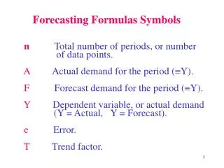
Forecasting Formulas Symbolsn Total number of periods, or number of data points.A Actual demand for the period (Y).F Forecast demand for the period (Y). Y Dependent variable, or actual demand (Y = Actual, Y = Forecast).e Error.T Trend factor.
C Cyclical factor.S Seasonal factor.Y Forecast dependent variable.a Y intercept.b Slope of the line. Alpha. The desired response rate, or smoothing constant.
(P) Probability.P Mean proportion of a large sample.Sigma standard deviation of the population.x Independent variable. y Dependent variable data point.
tMean of the error for a time interval.tError for a single time period. ZValue from normal distribution (i.e. number of standard deviation from the expected distribution).SStandard deviation of the errors.
R2 Coefficient of determination (The percentage of exploised, eliminated and removed variances).Z MAD Mean absolute deviation. I Index. mu population mead.
Sx = (X-X)2/(n-1) Sample standard deviation of X. x = (X- )2/N Population standard deviation of X. Syx = (Yt-Yt)2/(n-r)Standard deviation of estimate standard deviation of forecast errors. (n = number of observations, r = smoothing) or regression (2) (a & b) indicators).
Syx = S Standard deviation of estimate standard deviation of the Errors.t = At - FtForecast error for period t = actual demand for period t less the (should be ~ ND (0,low) forecast demand for period t.Ft = Ft-1 + (At-1 – Ft-1) The exponentially smoothed forecast for period t = the exponentially smoothed forecast for the prior period + the smoothing constant times (the actual for the prior period less the forecast for the prior period).
Yt = a + bt Forecast: Simple Linear Trend.Yt = a + bt + ct2 Forecast: Quadratic Trend.Yt = T CI SI I Decomposition model: Forecast value = Trend times cyclical indicators times seasonal indicator times irregular indicator.Yt = T SI Simple Decomposition model: Forecast value = Trend times seasonal indicator.
2 x+y = 2 x +2 yStandard deviation squared for x + y = the standard deviation of x + the standard deviation of y. x+y = x +yPopulation mean for x + y = the mean of x + the mean of y. et - 0 TS = Tracking signal = the totalMAD of errors/MAD.
t - 0Z = Z – value for Serrors = the mean of the errors for a time interval over the standard deviation of the errors. APE MAPE = n
MAD = 0.8SeMean absolute deviation = 0.8 times the standard deviation of the forecast errors.S = MAD (1.25)Standard deviation of the forecast errors = mean absolute deviation times 1.25.t = 0 Z SConfidence interval for errors = times standard deviation of the forecast errors.
A - FAPE= |A Absolute value of actual less forecast divided by actual.Syx 2 R2 = 1 - sy 2The coefficient of se2 determination = 1 - sy2
s y 2 - s 2R2 = The coefficient of s y 2 determination.