Download
1 / 40
400 likes | 574 Views
Tide Simulation Using Regional Ocean Modeling System (ROMS). Xiaochun Wang. a b. a. a b. a b. c. Co-author: Yi Chao, Zhijin Li, John Farrara, Changming Dong, James McWillams. c. Contributions from: K. Matsumoto, C. K. Shum, Y. Wang, Quoc Vu

E N D
Tide Simulation Using Regional Ocean Modeling System (ROMS) Xiaochun Wang a b a a b a b c Co-author: Yi Chao, Zhijin Li, John Farrara, Changming Dong, James McWillams c Contributions from: K. Matsumoto, C. K. Shum, Y. Wang, Quoc Vu Discussions with: L. Rosenfeld, J. Paduan, M. Foreman Fifteen Years of Progress in Radar Altimetry, Venice 2006 a: Jet Propulsion Lab/California Institute of Technology b: Raytheon, ITSS c: IGPP, University of California Los Angeles
Three Level Nested ROMS San Francisco Monterey Bay Los Angeles 3-Level Nested Model Grid Size Time Step Res. L0: 85*170*32 900s 16.5km L1: 95*191*32 300s 5.3km L2: 83*179*32 100s 1.8km Monterey Bay 16 Processors on SGI Altix 3000 1 hour integration takes 1min cpu time.
Boundary Conditions SSH: Chapman condition Tangential Barotropic Velocity: Oblique radiation Normal Barotropic Velocity: Flather condition • Open Boundary Condition • Closed Boundary Condition SSH: Zero gradient Tangential Velocity: Free slip Normal Velocity: Zero Tide SSH and transport are from the barotropic tide data assimilation system of Oregon State University (TPXO.6 Egbert et. al, 1994, 2002). Atmospheric Forcing: Hourly wind stress and heat flux.
Comparison with T/P Tide Estimation Away from the coast Root of Summed Squares 3.45cm Courtesy of Dr. K Matsumoto, and C.K. Shum, Y Wang. <6% of M2 amplitude
Comparison with Tide Gauges RSS 3.51cm Monterey Domain 3 Gauges RSS 5.41cm US SW Coast Domain 10 Gauges Along the coast <10% of M2 amplitude
Baroclinic Tide Theory Generation Baroclinic Tide Forcing Subscript i : Baroclinic Subscript 1: Barotropic Stratification, Bathymetry, Barotropic tide flux Energetics E: Baroclinic tide energy CgE: Baroclinic tide energy flux G: Forcing D: Dissipation Baines (1982), Gill(1982)
Surface Tide Current Ellipses (M2) Major Axis: 5.80cm/s Major Axis: 4.24cm/s Major Axis Inclination Minor Axis Phase Blue: Counter-clock Green: Clockwise
Surface Current Ellipses at K1 Frequency Major Axis: 8.66 cm/s Major Axis: 5.63cm/s
Diurnal Surface Current Variability Mainly Caused by Wind Hourly wind+Tide (5.63cm/s) Monthly wind+Tide (0.98cm/s)
Baroclinic Tide Energy J/m^2 Depth Integrated Energy Depth Integrated Forcing Energy level comparable with observation Energy can be generated outside the bay
Baroclinic Tide Energy Flux N E S W/M*M Baroclinic tide energy can get into the bay through the northern path and southern path. Depth Integrated Baroclinic Tide Flux
Baroclinc Tide around Mendocino Escarpment J/m^2 m^/s^2 Baroclinic Tide Forcing Energy Flux Baroclinic Tide Energy
Summary • ROMS can simulate barotropic tide reasonably well in Monterey Bay. • The general pattern of sea surface current is comparable with high frequency radar observation. • Surface current variability at diurnal frequency is mainly caused by the wind. Future Work: Continue to improve baroclinic tide solution with better stratification and bathymetry.
Baroclinic Tide Forcing Term Based on TPXO6.0 global barotropic tide solution Stratification is not included
EXP1 EXP2 EXP3 EXP4 Exp1: Climatlogy Exp2: I-year spinup Exp3: Data Assimilation + Hourly Wind Exp4: Data Assimilation + Monthly Wind Stratification !
Baroclinic Tide Forcing M^2/S^2
Baroclinic Tide Theory Generation Baroclinic Tide Forcing Subscript i : Baroclinic Subscript 1: Barotropic Energetics Baroclinic tide energy Baroclinic energy flux Baines (1982) Gill(1982) G: Forcing, D: Dissipation
Tide Solution in Nested ROMS (M2) Tide constituents used: M2 K1 O1 S2 N2 P1 K2 Q1
Baroclinic Tide Energy K1 M2
Internal Tide Forcing Term Stratification Bathymetry Barotropic Tide Tide Frequency Where the internal tide energy generated?
Nested Tide Solution for One Station Tide solution is improved in finer resolution model domain.
Energy Flux along NSE Section (M2) Internal Tide ( 5.33 *10**6 W) Barotropic Tide (1.19*10**8 W)
Energy Flux along NSE Section (K1) Internal Tide (-5.17 *10**3 W) Barotropic Tide (5.24*10**3 W)
Quadratic Bottom Drag Coefficient 3.e-3 1.e-3 30e-3 100e-3 Tide solution is more robust in OGCMs than in barotropic models.
Spatial Comparison (M2 K1 O1 S2) ROMS SSH TPXO (SSH) M2 K1 K1 M2 O1 O1 S2 S2
Spatial Comparison (Vbar) ROMS TPXO
Spatial Comparison (Ubar) ROMS TPXO
RMS of ROMS (L1) and TPXO SSH Ubar Vbar Difference of SSH is small. Difference of transport is large.
Influence of Boundary Condition U V only SSH only SSH + U V Tidal Solution is a combined effect of boundary conditions.
Comparison with Tide Gauges (Amp) RSS: 5.41cm RSS: 2.72cm Coastal region
Comparison with Tide Gauges (Phase) M2 K1 O1 S2 N2 P1 K2 Q1 Blue: Tide Gauge Green: ROMS Red: TPXO
Comparison with Tide Gauges (Amp) RSS: 5.41cm M2 K1 O1 S2 N2 P1 K2 Q1 RMS 4.59 1.29 0.92 2.00 0.64 0.93 0.54 0.29 Coastal region, 10 stations.
Comparison with Tide Gauges (Phase) M2 K1 O1 S2 N2 P1 K2 Q1 Blue: Tide Gauge Green: ROMS M2 K1 O1 S2 N2 P1 K2 Q1 RMS 3.42 2.39 3.75 4.06 2.53 5.10 3.08 7.28
Comparison with Tide Gauges RMS of one month sea surface height from model and 10 tide gauges.