Download
1 / 36
360 likes | 388 Views
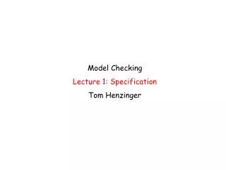
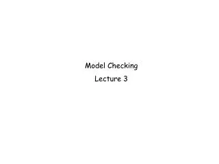
Model Checking Lecture 3 Tom Henzinger. Model-Checking Problem. I |= S. System model. System property. System Model. -state-transition graph -weak or strong fairness constraints. System Properties. Temporal logics -STL (finite runs) : , U

E N D
Model Checking Lecture 3 Tom Henzinger
Model-Checking Problem I |= S System model System property
System Model -state-transition graph -weak or strong fairness constraints
System Properties Temporal logics -STL (finite runs) : , U -CTL (infinite runs) : , U, -LTL (infinite traces) : , U Automata -specification automata (trace containment) -monitor automata (trace emptiness) -simulation automata (relation on finite runs)
Acceptance Conditions -finite automata: -Buchi automata: -coBuchi automata: -Streett automata: ( ) -Rabin automata: ( )
Response specification automaton : (a b) assuming (a b) = false s1 a b s2 s0 b a s3 Buchi condition { s0, s3 }
Response monitor automaton : (a b) assuming (a b) = false true a b s0 s1 s2 Buchi condition { s2 }
a a a s1 s0 Buchi condition { s0 } No coBuchi condition Streett condition { ({s0,s1}, {s0}) } Rabin condition { (, {s0}) }
a a a s1 s0 No Buchi condition coBuchi condition { s0 } Streett condition { ({s1}, ) } Rabin condition { ({s1}, {s0,s1}) }
a a a s1 s0 a s2 Buchi condition { s2 }
-Buchi and coBuchi automata cannot be determinized -Streett and Rabin automata can be determinized nondeterministic Buchi = deterministic Streett = deterministic Rabin = nondeterministic Streett = nondeterministic Rabin = omega-regular [Buchi 1960]
Omega-automata are strictly more expressive than LTL Omega-automata: omega-regular languages LTL: counter-free omega-regular languages
Omega-automata: omega-regular languages = second-order theory of monadic predicates & successor= omega-regular expressions LTL: counter-free omega-regular languages = first-order theory of monadic predicates & successor= star-free omega-regular expressions
Structure of the Omega-Regular Languages Streett = Rabin Buchi coFinite Finite coBuchi
Structure of the Counter-free Omega-Regular Languages finite boolean combinations of and
The location of a linear-time property in the Borel hierarchy indicates how hard (theoretically as well as conceptually) the corresponding model-checking problem is.
finite boolean combinations of and weak fair safety response strong fair
Safety: • -solve: STL (U model checking), finite monitors ( emptiness) • -algorithm: reachability (linear) • Response under weak fairness: • -solve: weakly fair CTL ( model checking), Buchi monitors ( emptiness) • -algorithm: strongly connected components (linear) • Liveness: • -solve: strongly fair CTL, Streett monitors ( () emptiness) • -algorithm: recursively nested SCCs (quadratic)
From specification automata to monitor automata: determinization (exponential) + complementation (easy) From LTL to monitor automata: complementation (easy) + tableau construction (exponential) Simulation automata: preorder refinement (quadratic)
Five Algorithms • Reachability • Strongly connected components • Recursively nested SCCs • Tableau construction • Preorder refinement • Streett determinization
Finite Emptiness Given: finite automaton (S, S0, , , FA) Find: is there a path from a state in S0 to a state in FA ? Solution: depth-first or breadth-first search
Application 1: STL model checking Application 2: finite monitors
Buchi Emptiness Given: Buchi automaton (S, S0, , , BA) Find: is there an infinite path from a state in S0 that visits some state in BA infinitely often ? Solution: 1. Compute SCC graph by depth-first search 2. Mark SCC C as fair iff C BA 3. Check if some fair SCC is reachable from S0
Application 1: CTL model checking over weakly-fair transition graphs (note: really need multiBuchi) Application 2: Buchi monitors
Streett Emptiness Given: Streett automaton (S, S0, , , SA) Find: is there an infinite path from a state in S0 that satisfies all Streett conditions (l,r) in SA ? Solution: check if S0 RecSCC (S, , SA)
function RecSCC (S, , SA) : X := for each C SCC (S, ) do F := if C then for each (l,r) SA do if C r then F := F (l,r) else C := C \ l if F = SA then X := X pre*(C) else X := X RecSCC (C, C, F) return X
Complexity n number of states m number of transitions s number of Streett pairs Reachability: O(n+m) SCC: O(n+m) RecSCC: O((n+m) · s2)
Application 1: CTL model checking over strongly-fair transition graphs Application 2: Streett monitors
Tableau Construction Given: LTL formula Find: Buchi automaton M such that L(M) = L() [Fischer & Ladner 1975; Manna & Wolper 1982]
Fischer-Ladner Closure of a Formula Sub (a) = { a } Sub () = { } Sub () Sub () Sub () = { } Sub () Sub () = { } Sub () Sub (U) = { U, (U) } Sub () Sub () | Sub () | = O(||)
s Sub () is consistent iff -if () Sub () then () s iff s and s -if () Sub () then () s iff s -if (U) Sub () then (U) s iff either s or s and (U) s
Tableau M = (S, S0, , , BA) S ... set of consistent subsets of Sub () s S0 iff s s t iff for all () Sub (), () s iff t (s) ... conjunction of atomic observations in s and negated atomic observations not in s For each (U) Sub (), BA contains { s | s or (U) s }
Size of M is O(2||). CTL model checking: linear / quadratic LTL model checking: PSPACE-complete
Preorder Refinement Given: state-transition graph (Q, , A, [ ] ) Find: for each state q Q, the set sim(q) Q of states that simulate q [ Bloom & Paige; H, H, & Kopke 1995 ]
for each t Q do sim(t) := { u Q | [u] = [t] } while there are three states s, t, u such that t s & u sim(t) & sim(s) post(u) = do sim(t) := sim(t) \ {u} {assert if u simulates t, then u sim(t) }