Download

1 / 22
230 likes | 338 Views
Sensitivity and Resolution of Tomographic Pumping Tests in an Alluvial Aquifer. Geoffrey C. Bohling Kansas Geological Survey 2007 Joint Assembly Acapulco, Mexico, 23 May 2007. Simultaneous analysis of multiple tests (or stresses) with multiple observation points

E N D
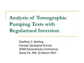
Sensitivity and Resolution of Tomographic Pumping Tests in an Alluvial Aquifer Geoffrey C. Bohling Kansas Geological Survey 2007 Joint Assembly Acapulco, Mexico, 23 May 2007
Simultaneous analysis of multiple tests (or stresses) with multiple observation points Information from multiple flowpaths helps reduce nonuniqueness Presented regularized inversion before Now going back to look at sensitivity and resolution Hydraulic Tomography Bohling
Highly permeable alluvial aquifer (K ~ 1.5x10⁻³ m/s) Many experiments over past 19 years Induced gradient tracer test (GEMSTRAC1) in 1994 Hydraulic tomography experiments in 2002 Various direct push tests over past 7 or 8 years Field Site (GEMS) Bohling
Field Site Stratigraphy From Butler, 2005, in Hydrogeophysics (Rubin and Hubbard, eds.), 23-58 Bohling
Tomographic Pumping Tests Bohling
Transient Fit, Gems4S Using K field for a = 0.025 with Ss = 9x10⁻⁵ m-1 Bohling
Drawdowns Relative to 3N Bohling
Sensitivity and Resolution Analysis • Forward simulation with 2D radial-vertical flow model in Matlab (vertical wedge) • Common 20 x 14 (1.5 m x 0.76 m) Cartesian grid of K,Ss values mapped into radial grid for each test (K=1x10⁻³ m/s, Ss=1x10⁻⁴ m-1) • Finite-difference Jacobian matrix, J • Model resolution matrix R = J†J, where J† is pseudo-inverse based on SVD • Transient and steady-shape analyses Bohling
Drawdown Sensitivity, Test 7, Gems4N K1, S1: r<10.3 m K2, S2: r>10.3 m S1 influences only early time data Later: Changes in drawdown controlled by K2, K1 and S2 together contribute constant term Bohling
Drawdown Difference Sensitivity Looking at sensitivity of drawdown differences relative to 3N Almost entirely controlled by K1, that is, K within region of investigation (ROI) for these tests Bohling
Sum Squared Sensitivity, All Tests Sum of squared sensitivity of drawdown to K, Ss in each cell over all 23 tests, 6 obs points, 1-900 s Normalized sensitivities, so comparable Note difference in scales Bohling
Singular Values of Jacobian, Transient 560 parameters: 280 K, 280 Ss Larger singular values associated with better resolved combinations of parameters (eigenvectors) Smaller singular values with more poorly resolved combinations R = J†J = VpVp’ Bohling
Resolution, First 66 Eigenvectors R = 1 for perfectly resolved cells, 0 for unresolved Leading eigenvectors dominated by K in ROI Essentially no contribution of Ss to leading eigenvectors Bohling
Resolution, First 145 Eigenvectors With 145 eigenvectors, resolve K in ROI quite well Some resolution of Ss in ROI (max R values of about 0.61) Properties outside ROI much harder to resolve Bohling
K Sensitivity, Transient and Steady-Shape Root mean squared sensitivity to compensate for differing numbers of observations Similar patterns, but steady-shape focuses sensitivity on ROI Bohling
Singular Values of Jacobian, Steady-Shape Jacobian for 280 K values Much clearer behavior than transient: Eigenvectors past first 115 represent unresolvable parameter combinations Bohling
K Resolution, Transient and Steady-Shape Transient result using first 145 eigenvectors, as before Steady shape using first 115 eigenvectors So, steady shape resolution similar to “dominant” transient resolution Bohling
Conclusions • Transient analysis provides good resolution of K in ROI, some resolution of Ss in ROI • Parameter variations outside ROI difficult to resolve • Steady shape analysis focuses sensitivity on K in ROI and reduces or eliminates sensitivity to more poorly resolved parameters (K outside ROI, Ss anywhere) Bohling
Acknowledgment s • Field effort led by Jim Butler with support from John Healey, Greg Davis, and Sam Cain • Support from NSF grant 9903103 and KGS Applied Geohydrology Summer Research Assistantship Program Bohling
Regularizing w.r.t. Stochastic Priors Second-order regularization – asking for smooth variations from prior model Fairly strong regularization here ( = 0.1) Best 5 fits of 50 Bohling