Download
1 / 57
570 likes | 687 Views
Zero-Knowledge Proof Systems. Slides by Roel Apfelbaum & Eti Ezra. Enhanced by Amit Kagan . Adapted from Oded Goldreich’s course lecture notes. 17.1. Notation.

E N D
Zero-Knowledge Proof Systems Slides by Roel Apfelbaum & Eti Ezra. Enhanced by Amit Kagan. Adapted from Oded Goldreich’s course lecture notes.
17.1 Notation Let A and B be a pair of ITMs (interactive TMs). <A,B>(x) is the random variable representing the (local) output of B when interacting with machine A on common input x, when the random-input to each machine is uniformly and independently chosen.
Zero Knowledge (Definition) • Let (P,V) be an interactive proof system for some language L. We say that (P,V), actually P, is zero-knowledge if for every probabilistic polynomial-time ITM V* there exists a probabilistic polynomial-time machine M* s.t. for every xL holds {<P,V*>(x)}xL {M*(x)}xL • Machine M* is called the simulator for the interaction of V* with P.
Perfect Zero Knowledge (Definition) Let (P,V) be an interactive proof system for some language L. We say that (P,V), actually P, is perfect zero-knowledge (PZK) if for every probabilistic polynomial time ITM V* there exists a probabilistic polynomial-time machine M* s.t. for every xL thedistributions {<P,V*>(x)}xL and{M*(x)}xL are identical, i.e.,{<P,V*>(x)}xL {M*(x)}xL
Example A trivial simulator for <P,V> • Let V be a verifier that satisfies the definition of IP - when xL, V accepts with probability close to 1, and when xL, Vaccepts with probability close to 0. • Let M be the simulator that always accepts. • When xL the distributions <P,V>(x) and M(x) are very close.
Statistically close distributions (Definition) The distribution ensembles {Ax}xLand{Bx}xL are statistically close or have negligiblevariation distance if for every polynomial p(•) there exits integer N such that for every xL with |x| N holds: |Pr [Ax = ] – Pr [Bx = ]| 1/p(|x|).
Statistical zero-knowledge (Definition) Let (P,V) be an interactive proof system for some language L. We say that (P,V), actually P, is statistical zero knowledge(SZK)if for every probabilistic polynomial time verifier V* there exists a probabilistic polynomial-time machine M* s.t. the ensembles {<P,V*>(x)}xLand {M*(x)}xLarestatistically close.
Computationally indistinguishable (Definition) Two ensembles {Ax}xLand{Bx}xLare computationally indistinguishable if for every probabilistic polynomial time distinguisher D and for every polynomial p(•) there exists an integer N such that for everyxL with |x| N holds |Pr [D(x,Ax) = 1] – Pr [D(x,Bx) = 1]| 1/p(|x|)
Computational zero-knowledge (Definition) Let (P,V) be an interactive proof system for some language L. (P,V), actually P, is computational zero knowledge (CZK) if for every probabilistic polynomial-time verifier V* there exists a probabilistic polynomial-time machine M* s.t. the ensembles {<P,V*>(x)}xL and {M*(x)}xLare computationally indistinguishable.
Lemma: BPP PZK Proof: SinceLBPP,V can be set to a probabilistic polynomial time machine that decides L. P is deterministic and never sends data to V. Clearly <P,V> is an interactive proof system (completeness and soundness conditions hold). (P,V) is PZK because for every V*: {<P,V*>(x)}xL {V*(x)}xL V* is a simulator for itself!
17.2 Graph isomorphism is in Zero-Knowledge • ISO := {(<G1>,<G2>) | G1 G2} Construction (ZK IP for ISO): • Common input: G1 = (V1, E1), G2 = (V2, E2). • Let be anisomorphism between G1andG2. Suppose that |V1| = |V2| = n.
Construction (cont.) (P1): P selects a random permutation over V1, constructs the set F where F := { ((u), (v)) : (u,v) E1 }, and sendsH = (V1,F)to V. (V1): V gets G’ = (V’,E’) from P. V selects R{1,2} and sends it to P. P is supposed to answer with an isomorphism between G and G’.
Construction (cont.) (P2): If =1, thensend = toV. Otherwise, send = -1to V. (V2):If is an isomorphism between G and G’ then V outputs 1, otherwise it outputs 0.
Construction (diagram) Prover Verifier R Sym([n]) H G1 R{1,2} H If=1, send = , otherwise = -1 Accept iff H = (G)
3 2 4 G2 4 5 5 1 G1 2 1 3 An example: • Common input: two graphs G1 and G2. Only P knows.
= -1 4 G2 2 5 3 2 5 1 1 3 H 4 2 4 G1 5 3 1 An example (cont.) V sends =2 to P. P sends Hto V. V gets and accepts. Only P knows.
Theorem: Graph isomorphism is in Zero-Knowledge Theorem 1: The construction above is a perfect zero-knowledge interactive proof system (with respect to statistical closeness).
Proof of Theorem 1 Completeness: If G1 G2 , V always accepts. First, G’=(G1). If =1 then = , Hence: (G) = (G1) = (G1) = G’ . If =2 then = -1, Hence: (G) = -1(G2) = (G1) = G’ . And hence V alwaysaccepts whenG1 G2 .
Proof of Theorem 1 (cont.) Soundness: Let P* be any prover. If it sends to V a graph not isomorphic neither to G1 nor to G2, then there is no isomorphism betweenG and G’. Hence V rejects. W.l.o.g, if G’ G1 then P* can convince V with probabilityat most 1/2 (V selects{1,2} uniformly). Hence: when G1 and G2 are non-isomorphic: Pr [<P*,V>(<G1>,<G2>) = accept] 1/2
Zero Knowledge(Construction of a simulator) • Let V*be any polynomial-time verifier, and let q(•) be a polynomial bounding the running time of V*. • M* selects a string rR{0,1}q(|x|). 01100…………011 r =
Meaning: (2)=1 = 2 4 2 5 G2 5 1 1 G’’ 3 2 3 4 Construction of a Simulator (cont.) • M* selects R{1,2}. • M*selects a random permutation over V. • M*constructs G’’=(G). =
input-tape random-tape = 2 x r G’’ message-tape Construction of a Simulator (cont.) • M* runs V* with the latter’s strings set as follows: • Denote as V*‘s output. If it were the case that ≠ , then the simulation would fail. • M*halts with output (x,r,G’’,).
Proof of Theorem 1 (cont.) Definition: Let (P,V) be an interactive proof system for L. (P,V) is perfect zero-knowledge by view if for every probabilistic polynomial-time verifier V* there exists a probabilistic polynomial time machine M* s.t. for every xL holds:{view<P,V*>(x)}xL {M*(x)}xL where view<P,V*>(x) is the final view of V* after running <P,V*> on input x. view = all the data a machine possesses
Proof of Theorem 1 (cont.) Lemma:An interactive proof system is perfect zero-knowledge iff it is perfect zero knowledge by view. Proof: Let M* satisfy: {view<P,V*>(x)}xL {M*(x)}xL for everyxL. M* has on its work-tape the final view of V*. Hence, it is able to perform the last step of V* and output the result. And so the modified M*(x) is identical to <P,V*>(x).
Proof of lemma (cont.) Let M* satisfy: {<P,V*>(x)}xL {M*(x)}xL . For a particular V*, let us consider a verifier V**that behaves exactly like V*, but outputs its whole view (at the end). There is a machine M** s.t. {<P,V**>(x)}xL {M**(x)}xL
Proof of Theorem 1 (cont.) Lemma:Let x=(G1,G2)ISO. Then for every string r, graph H and permutation , it holds that: Pr [view<P,V*>(x) = (x,r,H,)] = Pr [M*(x) = (x,r,H,) | M*(x) ] Proof: Let m* describe M* conditioned on its not being . Define the 2 random variables: 1.v(x,r) - the last 2 elements of view(P,V*)(x) conditioned on the second element equals r. 2. (x,r) - the same with m*(x).
Proof of lemma (cont.) Let v*(x,r,H) denote the message sent by V* for a fixedr and an incoming message H. We will show that v(x,r) and (x,r) are uniformly distributed over the set: Cx,r := {(H,): H=(Gv*(x,r,H)) } While running the simulator we have H=(G), and only the pairs satisfying =v*(x,r,H) lead to an output. Hence: Pr((x,r)=(H,)) = { 1/|V1|! if H=(Gv*(x,r,H)) { 0 otherwise
Proof of lemma (cont.) Consider v(x,r): v(x,r) = { ((G1),) if v*(x,r,(G1))=1. { ((G2),-1) otherwise. For each H (which is isomorphic to G1): Pr((x,r)=(H,)) = { 1/|V1|! if =1-v*(x,r,H) { 0 otherwise Observing that H=(Gv*(x,r,H)) iff=1-v*(x,r,H) and hence the lemma follows.
Proof of Theorem 1 (cont.) Corollary:view<P,V*>(x) and M*(x) are statistically close. Proof: A failure is output with probability 1/2. If the simulator returns steps P1-P2 of the construction |x| times and at least once at step P2=, then output (x,r,G’’,). If in all |x| trials , then output rubbish. Hence, we got a statistical difference of 2-|x|, and so the corollary follows.
17.3 Zero-Knowledge for NP • Reminder:NP is like IP with 1/2 round. • We can define NP-ZK as ZK with 1/2 round,but it would be equivalent to BPP: • Lemma:If L admits a zero-knowledge NP-proof system, then LBPP. • Proof:The simulator for <P,V> accepting L is a BPP machine.
1 2 3 4 1 5 2 3 4 5 G3C • Common Input: A graph • Prover can color the graph using 3 colors. • Prover must keep the coloring secret.
1 2 3 4 1 5 2 3 4 4 3 5 1 2 5 G3C is in Zero-Knowledge Construction (ZK IP for G3C): • Prover chooses a random color permutation. • Prover puts all the vertices` colors inside envelopes. • And sends them to the verifier.
1 2 3 4 5 1 2 3 4 5 G3C is in ZK (cont.) • Verifier receives envelopes supposedly containing a legal 3-coloring of the graph • Verifier chooses an edge at random. • And asks Prover to open the 2 envelopes.
1 2 3 4 5 1 2 3 G3C is in ZK (cont.) • Prover opens the envelopes, revealing the colors. • Verifier accepts if the colors are different.
Formally, • G = (V,E) is 3-colorable if there exists a mapping so that for every . • Let be a 3-coloring of G, and let be a permutation over {1,2,3} chosen randomly. • Define a random 3-coloring. • Put each (v) in a box with v marked on it. • Send all the boxes to the verifier.
Formally, (cont.) • Verifier selects an edge at random asking to inspect the colors. • Prover sends the keys to boxes u and v. • Verifier uses the keys to open the boxes. • If the Verifier finds 2 different colors from {1,2,3} - Accept. • Otherwise - Reject.
1 2 n (1) (2) (n) P V P V Keyu , keyv P V G3C (diagram)
The construction is in ZK: • Completeness:If G is 3-colorable and both P and V follow the rules, V accepts. • Soundness:Suppose G is not 3-colorable and P* tries to cheat. Then at least one edge (u,v) will be monochromatic: (u) = (v).V hence picks a bad edge with probability 1/|E|, which can be increased to 2/3 by repeating the protocol sufficiently many times.
Zero Knowledge(Construction of a simulator) • Let V*be any polynomial-time verifier, and let q(•) be a polynomial bounding the running time of V*. • M* selects a string rR{0,1}q(|x|). 11010…………110 r =
Construction of a Simulator (cont.) • M*selectse’=(u’,v’) R E. • M*sends to V* boxes filled with garbage, except for the boxes of u’ and v’, colored as follows: C R {1,2,3} d R {1,2,3}\{c} c d u’ v’ • If V* picks (u’,v’), M* sends V* their keys and the simulation is completed. • Otherwise, the simulation fails.
Analysis of the Simulation For every GG3C, the distribution of m*(<G>) = M*(<G>) | (M*(<G>) ) is identical to <P,V*>(<G>). Since V* can’t tell e’ from other edges by looking at the boxes, he picks e’ with probability 1/|E|, which can be increased to a constant by repeating M* sufficiently many times. So if the boxes are perfectly sealed, G3CPZK.
Commitment Scheme • Digital implementation of a “sealed box”. • Commitment Scheme is a 2-phase protocol satisfying: • Secrecy: At the end of phase #1, R (Receiver) can’t tell what value is being sent. • Unambiguity: Given the transcript of phase #1, there’s at most one value R may accept as legal at phase #2.
Commitment Scheme • Denote S(s,) the message S (Sender) sends to R when committing itself to bit and his random coins are s. • Secrecy means S(s,0) and S(s,1) are computationally indistinguishable. • Unambiguity means R can’t be fooled to think S(s,0) = S(s’,1) for any s and s‘.
Commitment Scheme • Unambiguity:Denote by r the coin tosses of R, and by View(R) everything known to R after having received m (S(s,) in this case) and tossed r. Denote by View(S) everything known to S from s and.Then for all but a negligible fraction of r‘s there’s no such m for which there are s and s‘ s.t.View(S)=(s,0) and View(R)=(r,m)and View(S)=(s’,1) and View(R)=(r,m)
Commitment Scheme Construction: • f:{0,1}n {0,1}n is one-way permutation.b:{0,1}n {0,1} is its hard-core bit. • Swants to send v{0,1} to R. • Phase #1:S selects sR{0,1}n and sends(f(s), b(s)v) to R, who stores them as (,) respectively. • Phase #2:S sends s as key. R calculates v = b(s), and accepts if f(s) = . Otherwise rejects.
Commitment Scheme • Proposition: This protocol is a bitcommitment scheme.Proof: • Secrecy: For every receiver R* consider the distribution ensembles<S(0),R*>(1n) = (f(s),b(s))and <S(1),R*>(1n) = (f(s),b(s)1)b(s) is unpredictable given f(s) and so the two ensembles are computationally indistinguishable.
Commitment Scheme • Unambiguity follows from f being one-to-one.
17.8 G3C+Commitment Scheme • Proposition:G3C that uses bit commitment schemes instead of “magic boxes” is computational zero-knowledge.Proof: • Completeness:P can convince V by sending the “right keys” of the commitment schemes for the colors of the vertices V selected.
G3C + Commitment Scheme • Soundness: Commitment scheme unambiguity ensures soundness is still satisfied.P may succeed to cheat V on phase #2 of commitment(in addition to the possibility that V won’t select a badly colored edge).However, this increases only by a little the probability of accepting GG3C.
G3C + Commitment Scheme • Computational Zero-Knowledge:Let M* be the simulator for V* from the previous proof.1) Pr[M*(x)=] is still small enough.2) The ensembles of {m*(<G>)}GG3C and {<P,V*>(<G>)}GG3C are computationally indistinguishable.