Download
1 / 30
300 likes | 403 Views
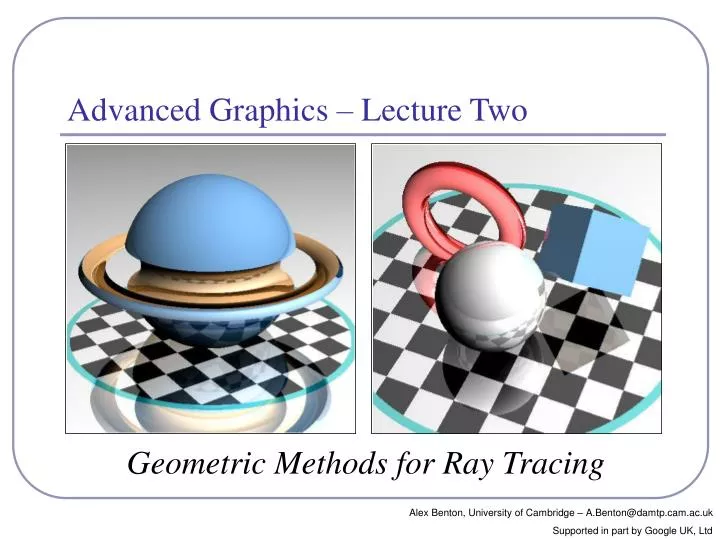
Geometric Methods for Ray Tracing. Advanced Graphics – Lecture Two. Alex Benton, University of Cambridge – A.Benton@damtp.cam.ac.uk Supported in part by Google UK, Ltd. Ray tracing revisited. (Slide from Neil Dodgson’s Computer Graphics and Image Processing notes, Cambridge University.).

E N D
Geometric Methods for Ray Tracing Advanced Graphics – Lecture Two Alex Benton, University of Cambridge – A.Benton@damtp.cam.ac.uk Supported in part by Google UK, Ltd
Ray tracing revisited (Slide from Neil Dodgson’s Computer Graphics and Image Processing notes, Cambridge University.)
The basic algorithm is straightforward Much room for subtlety Refraction Reflection Shadows Anti-aliasing Blurred edges, depth-of-field effects Ray tracing typedef struct{double x,y,z}vec;vec U,black,amb={.02,.02,.02}; struct sphere{ vec cen,color;double rad,kd,ks,kt,kl,ir}*s, *best,sph[]={0.,6.,.5,1.,1.,1.,.9, .05,.2,.85,0.,1.7,-1.,8.,-.5,1.,.5,.2,1.,.7,.3,0.,.05,1.2,1.,8.,-.5,.1,.8,.8, 1.,.3,.7,0.,0.,1.2,3.,-6.,15.,1.,.8,1.,7.,0.,0.,0.,.6,1.5,-3.,-3.,12.,.8,1., 1.,5.,0.,0.,0.,.5,1.5,};yx;double u,b,tmin,sqrt(),tan();double vdot(A,B)vec A ,B;{return A.x*B.x+A.y*B.y+A.z*B.z;}vec vcomb(a,A,B)double a;vec A,B;{B.x+=a* A.x;B.y+=a*A.y;B.z+=a*A.z;return B;}vec vunit(A)vec A;{return vcomb(1./sqrt( vdot(A,A)),A,black);} struct sphere*intersect(P,D)vec P,D;{best=0;tmin=1e30;s= sph+5;while(s-->sph)b=vdot(D,U=vcomb(-1.,P,s->cen)),u=b*b-vdot(U,U)+s->rad*s ->rad,u=u>0?sqrt(u):1e31,u=b-u>1e-7?b-u:b+u,tmin=u>=1e-7&&u<tmin?best=s,u: tmin;return best;}vec trace(level,P,D)vec P,D;{double d,eta,e;vec N,color; struct sphere*s,*l;if(!level--)return black;if(s=intersect(P,D));else return amb;color=amb;eta=s->ir;d= -vdot(D,N=vunit(vcomb(-1.,P=vcomb(tmin,D,P),s->cen )));if(d<0)N=vcomb(-1.,N,black), eta=1/eta,d= -d;l=sph+5;while(l-->sph)if((e=l ->kl* vdot(N,U= vunit(vcomb(-1.,P,l->cen))))>0&& intersect(P,U)==l) color=vcomb(e ,l->color,color);U=s->color; color.x*=U.x; color.y*=U.y;color.z*=U.z;e=1-eta* eta*(1-d*d);return vcomb(s->kt,e>0?trace(level,P,vcomb(eta,D,vcomb(eta*d-sqrt (e),N,black))):black,vcomb(s->ks,trace(level, P,vcomb(2*d, N,D)),vcomb(s->kd, color,vcomb(s->kl,U,black)))); }main(){printf("%d %d\n",32,32);while(yx<32*32) U.x=yx%32-32/2,U.z=32/2-yx++/32,U.y=32/2/tan(25/114.5915590261), U=vcomb(255., trace(3,black,vunit(U)),black),printf("%.0f %.0f %.0f\n",U);}/*minray!*/ Paul Heckbert’s ‘minray’ ray tracer, which fit on the back of his business card. (circa 1983)
Ray tracing • The ray tracing time for a scene is a function of(num rays cast) x(num lights ) x(num objects in scene) x (num reflective surfaces ) x(ray reflection depth) x … • Contrast to polygon rasterization: time is a function of the number of elements in the scene times the number of lights. (Scene from the realtime ray traced Quake 4)
The algorithm For each pixel on the screen, do: • Calculate ray from eye (O) through pixel (X) Set D = (X-O) / |(X-O)| Ray: R=O+tD • Find ray/primitive hit point (P) and normal (N) • Compute shadow, reflection, transparency rays; recursively call steps 2—4 • Calculate lighting of surface at point
Ray/polygon intersection O+tD Ray R=O+tD Poly P={v1,…,vn} N= (vn-v1)x(v2-v1) N•(O+tD-v1)=0 Nx(Ox+tDx-vx1) + Ny(Oy+tDy-vy1) + Nz(Oz+tDz-vz1)=0 NxOx+tNxDx-Nxvx1 + NyOy+tNyDy-Nyvy1 + NzOz+tNzDz-Nzvz1=0 tNxDx + tNyDy + tNzDz=Nxvx1+Nyvy1+Nzvz1-NxOx-NyOy-NzOz t = ((N•v1)-(N•O)) / (N•D) N D Oc
Point-in-nonconvex-polygon • Ray casting (1974) • Odd number of crossings = inside • Issues: • How to find a point that you know is inside? • What if the ray hits a vertex? • Best accelerated by working in 2D • You could transform all vertices such that the coordinate system of the polygon has normal = Z axis… • Or, you could observe that crossings are invariant under scaling transforms and just project along any axis by ignoring (for example) the Z component. • Validity proved by the Jordan curve theorem…
A B The Jordan curve theorem “Any simple closed curve C divides the points of the plane not on C into two distinct domains (with no points in common) of which C is the common boundary.” • First stated (but proved incorrectly) by Camille Jordan (1838 -1922) in his Cours d'Analyse. • Sketch of proof : (For full proof see Courant & Robbins, 1941.) • Show that any point in A can be joined to any other point in A by a path which does not cross C, and likewise for B. • Show that any path connecting a point in A to a point in B must cross C. C
The Jordan curve theorem on a sphere • Note that the Jordan curve theorem can be extended to a curve on a sphere, or anything which is topologically equivalent to a sphere. “Any simple closed curve on a sphere separates the surface of the sphere into two distinct regions.” A B
Point-in-nonconvex-polygon • Winding number (1980s) • The winding number of a point P in a curve C is the number of times that the curve wraps around the point. • For a simple closed curve (as any well-behaved polygon should be) this will be zero if the point is outside the curve, non-zero of it’s inside. • The winding number is the sum of the angles from vi to P to vi+1. • Caveat: This method is elegant but slow. Figure from Eric Haines’ “Point in Polygon Strategies”, Graphics Gems IV, 1994
Point-in-convex-polygon • Half-planes method • Each edge defines an infinite half-plane covering the polygon. If the point P lies in all of the half-planes then it must be in the polygon. • For each edge e=vi→vi+1: • Rotate each edge 90˚ CCW around N. • If eR•(P-vi) < 0 then the point is outside e. • Fastest known method. v… v… N vn v1 v2 v3 D O P vi+1 eR e vi
Barycentric coordinates B • Barycentric coordinates (t1,t2,t3) are a coordinate system for describing the location of a point P inside a triangle (A,B,C). • (t1,t2,t3) are the ‘masses’ to be placed at (A,B,C) respectively so that the center of gravity of the triangle lies at P. • Interestingly, (t1,t2,t3) are also proportional to the subtriangle areas. t1+t3 P t2 A t1 Q t3 C B t3 t1 t2 A t1 t3 C
Ray/sphere intersection Ray R=O+tD Sphere S={P | P•P=r2} (centered at the origin; radius r) (O+tD) • (O+tD) = r2 (Ox+tDx)2 + (Oy+tDy)2 + (Oz+tDz)2 = r2 (Ox2+Oy2+Oz2) + 2t(OxDx+OyDy+OzDz) + t2(Dx2+Dy2+Dz2) –r2 = 0 t2(D•D) + 2t(O•D) + (O•O)–r2 = 0 Solve the quadratic at your leisure… t = (-(O•D) ± √((O•D)2 - (D•D)((O•O)–r2))) / (D•D) And of course the normal is equal to the normalized point of intersection.
Ray/cylinder intersection Cylinder C={P | Px2+Py2=r2, Pz≥0, Pz≤h} (centered at the origin, aligned along the Z axis; height h; radius r.) (Ox+tDx)2+ (Oy+tDy)2 = r2 (Ox2+Oy2) + 2t(OxDx+OyDy) + t2(Dx2+Dy2) –r2 = 0 t = (-(OxDx+OyDy) ± √((OxDx+OyDy)2 - (Dx2+Dy2)(Ox2+Oy2–r2))) / (Dx2+Dy2) Normal is P without its Z component, normalized. Remember to test Z coordinate as well: if cylinder is capped, test the intersections with the Z=h and Z=0 planes.
Ray/cone intersection Cone C={P | Px2+Py2=(h-Pz)2r2 / h2, Pz≥0, Pz≤h} (Base centered on the origin; height h, apex at A=(0,0,h), radius r.) (Ox+tDx)2+ (Oy+tDy)2 = (h-Oz-tDz)2(r2/ h2) (Ox2+Oy2) + 2t(OxDx+OyDy) + t2(Dx2+Dy2) = (r2/ h2) ((h-Oz)2 – 2t(h-Oz)Dz + t2Dz2) t2(Dx2+Dy2–(r2/ h2)Dz2) + 2t(OxDx+OyDy + (r2/ h2)(h-Oz)Dz) + (Ox2+Oy2) – (r2/ h2) (h-Oz)2= 0 a = (Dx2+Dy2–(r2/ h2)Dz2) b = 2(OxDx+OyDy + (r2/ h2)(h-Oz)Dz) c = Ox2+Oy2– (r2/ h2) (h-Oz)2 t = (-b± √(b2-4ac)) / 2a Normal direction at P is N=(A–P) x P x (A–P). A N P
Ray/torus intersection • How about a torus? Define F(P)=(Px,Py,0) as a shortcut for projecting P to the XY plane. Then an equation for a torus T of major radius r, minus radius s, parallel to the XY plane and centered on the origin, would be T={P | P–(rF(P)/||F(P)||) = s} (The algebra to intersect this with a ray is relatively straightforward but far too verbose to present here. It does involve a quartic.) Normal direction at P is N= (P/s)–(rF(P) / s||F(P)||)
Quadrics • A quadric is a second-order surface given by an equation of the general form • Quadrics can represent elipsoids, paraboloids, hyperbolic paraboloids, cones… and other surfaces! • Ex: x2+y2+z2=1describes a sphere • Ex: x2+y2-z2=1describes a hyperboloid of one sheet • With quadrics you can generalize your primitives.
Primitives and world transforms • Given a primitive P and its transform S, is it more efficient to find the intersection in screen space, world space or object space? • Not screen space: the transform from camera to screen co-ordinates is not affine, specifically it is not angle-preserving. This would prevent many nice optimizations, such as fast bounding box tests. • Our maths aren’t optimized for world space; it would be nice to have each primitive encoded as statically as possible (ideally in assembler) with minimal parametrization.
Primitives and world transforms • Object space, then. • Find R = O+tD in object coords: • S is the local-to-world transform of P. • Invert S to find S-1, the world-to-local transform. • Define OL=S-1(O) and DL=S-1(D). • The local ray: RL = OL + t’DL • Solve for t’ and find the world hit point at S(RL(t’)). • Wyvill (1995) (Part 2, p.45) compares the floating-point ops required to hit a sphere with a ray in world or local coordinates. He found that it is actually 37% more efficient, per ray, to intersect in local space.
Primitives and world transforms • What about the normal? • If S is just a concatenated sequence of rotates and translates then the normal can be transformed by S as above. • Scales make things trickier. • To find the world-space normal, multiply the local normal by the transpose of the inverse of S: N=(S-1)T NL • Can ignore translations • For any rotation Q, (Q-1)T=Q • Scaling is unaffected by transpose, and a scale of (a,b,c) becomes (1/a,1/b,1/c) when inverted NL local T NW world
Optimizing first contact in hardware • To accelerate first raycast, don’t raycast: use existing hardware. • Tell OpenGL to write to an offscreen 32-bit buffer. • Set the color of each primitive to a pointer to that primitive. • Render your scene in gl with z-buffering and no lighting. • The ‘color’ value at each pixel in the buffer is now a pointer to the primitive under that pixel.
Constructive Solid Geometry • Constructive Solid Geometry (CSG) builds up complicated forms out of simple primitives. • These primitives are combined with basic boolean operations: add, subtract, intersect. CSG figure by Neil Dodgson
Constructive Solid Geometry • CSG models are difficult to polygonalize. • Issues include choosing polygon boundaries at edges; converting adequately from pure smooth primitives to discrete (flat) faces; handling ‘infinitely thin’ sheet surfaces; and others. • This is an ongoing research topic. • CSG models are well-suited to machine milling, automated manufacture, and ray-tracing.
Constructive Solid Geometry • CSG surfaces can be described by a binary tree, where each leaf node is a primitive and each non-leaf node is a boolean operation. • (What would the notof a surface look like?) Figure from Wyvill (1995) part two, p. 4
Constructive Solid Geometry Three operations: 1. Union 2. Intersection 3. Difference
Ray tracing CSG models • For each node of the binary tree: • Fire your ray r at A and B. • List in t-order all points where r hits A or B. • Label each intersection point with a quad of booleans (wasInA, isInA, wasInB, isInB), tracking transitions across the borders of the primitives. • Discard from the list all intersections which don’t matter to the current boolean operation. • Pass the list up to the parent node and recurse.
Ray tracing CSG models • All three boolean operations can be modeled with one state diagram. • For each operation, retain those intersections that transition into or out ofthe critical state(s). • Union: {In A | In B | In A and B} • Intersection: {In A and B} • Difference: {In A} In A and B Enter A Enter B Leave B Leave A In just A In just B Leave A Enter B Enter A Not in A or B Leave B
Ray tracing CSG models t2, t3 • Example: Difference (A-B) A B t1 t4 difference = ((wasInA != isInA) && (!isInB)&&(!wasInB)) || ((wasInB != isInB) && (wasInA || isInA))
References • Ray tracing and CSG • G. Wyvill, Practical Ray Tracing (parts 1 and 2), University of Otago, 1995 • Jordan curves • R. Courant, H. Robbins, What is Mathematics?, Oxford University Press, 1941 • http://cgm.cs.mcgill.ca/~godfried/teaching/cg-projects/97/Octavian/compgeom.html • Point-in-polygon • http://tog.acm.org/editors/erich/ptinpoly/ • http://mathworld.wolfram.com/BarycentricCoordinates.html