Download
1 / 101
1.08k likes | 1.43k Views
An Introduction to Multivariate Models. Sarah Medland. SGDP Summer School July 2010. Twin Model. Univariate Model Bivariate Model Multivariate Models. Hypothesised Sources of Variation. Topics of Discussion: Extensions to multiple variables (3 or more) Choosing between :

E N D
An Introduction to Multivariate Models Sarah Medland SGDP Summer School July 2010
Twin Model • Univariate Model • Bivariate Model • Multivariate Models Hypothesised Sources of Variation Topics of Discussion: • Extensions to multiple variables (3 or more) • Choosing between : Cholesky Decomposition Common Pathway model Independent Pathway model Path Diagrams Model Equations Matrix Algebra Path Tracing Rules Predicted Var/Cov from Model Observed Var/Cov from Data Structural Equation Modelling (SEM)
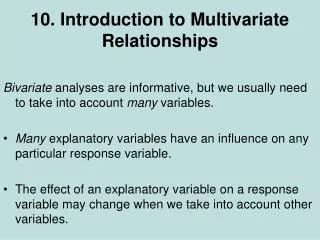
Multivariate analysis Univariate analysis:genetic and environmental influences on the variance of one trait Bivariate analysis:genetic and environmental influences on the covariance between two traits Multivariate analysis:genetic and environmental basis of the covariance between multiple traits
Multiple phenotypes Comorbid phenotypes Diagnostic subtypes (e.g. anxiety: panic, social, separation) Different dimensions (e.g. cognitive abilities) Different raters Self report, Mother-report, Teacher-report, Observational Longitudinal data Time-point 1, Time-point 2, Time-point 3, Time-point 4
Multivariate models Specific variance Common variance Why do these phenotypes covary?
Multivariate models Different models have different assumptions in the nature of shared causes among multiple phenotypes Cholesky Decomposition (Correlated factors solution) Genetic and environmental factors on different variables correlate Independent pathway model Specific and Common genetic and environmental causes Common pathway model Latent Psychometric factor mediates common genetic and environmental effects
Twin 2 A E A E A E A E A E A E A E A E Teacher Examiner Child Mum C C C C C C C C Cholesky Decomposition Twin 1 Teacher Examiner Child Mum Nvar Number of A, C and E Factors
The A Structure Twin 1 Twin 2 A A A A A A A A Teacher Examiner Child Mum Teacher Examiner Child Mum Number of A paths: [ nvar*(nvar+1) ] / 2 (4*5)/2 = 10
The C Structure Twin 1 Twin 2 Number of C paths: [ nvar*(nvar+1) ] / 2 (4*5)/2 = 10 Teacher Examiner Child Mum Teacher Examiner Child Mum C C C C C C C C
The E Structure Twin 1 Twin 2 E E E E E E E E Teacher Examiner Child Mum Teacher Examiner Child Mum Number of E paths: [ nvar*(nvar+1) ] / 2 (4*5)/2 = 10
Cholesky Decomposition Twin 1 Twin 2 rMZ= 1;rDZ= 0.5 E E E E E E E A A A E A A A A A Teacher Examiner Child Mum Teacher Examiner Child Mum C C C C C C C C rMZ/DZ = 1
Correlated factors solution am=am2 A E A E A E A E C C C C am aE aT aC Teacher Examiner Child Mum rA (M-T) rA (M-E) rA (T-E) rA (M-C) rA (T-C) rA (E-C)
Correlated factors solution cm=cm2 A E A E A E A E C C C C cm cE cT cC Teacher Examiner Child Mum rC (M-T) rC (M-E) rC (T-E) rC (M-C) rC (T-C) rC (E-C)
Correlated factors solution em=em2 A E A E A E A E C C C C em eE eT eC Teacher Examiner Child Mum rE (M-T) rE (M-E) rE (T-E) rE (M-C) rE (T-C) rE (E-C)
Correlated factors solution Assumptions • Each variable (e.g. Mother-rating) is influenced by a set of genetic, shared and non-shared environmental factors • 2. The factors associated with each variable are allowed to correlate with each other through rA, rC and rE • 3. Correlations among phenotypes are a function of rA, rC and rEand the standardized A, C and E paths connecting them
Independent & Common • Trait 1 Partition variance between variables: 1) Common variance: variance that is shared by all measured variables • Trait 2 • Trait 3 2) Specific variance: variance that is not shared by the measured variables S C C C C S S
What might common and specific variance represent? 1) Comorbid phenotypes: (e.g. anxiety subtypes) Common variance = general liability to emotional reactivity Specific variance = symptom-specific risks 2) Different raters: (e.g. mother, teacher, child reports) Common variance = pervasive liability to reported behaviour Specific variance = situation-specific behaviour
Independent pathway model rMZ= 1 rDZ = 0.5 Twin 1 Twin 2 rMZ / DZ = 1 A C E E C A Teacher Examiner Child Teacher Examiner Child Mum Mum C C C C A E A E A E A E C C C C E E A E E A A A
Independent pathway model Assumptions • Each variable (e.g. mother rating) has variation that is shared with other variables • “Common” genetic and environmental factors • Each variable is also influenced by unique variance not shared with other variables • “Specific” genetic and environmental factors • Covariation among phenotypes may be due to the same genetic or environmental causes
Independent pathway model Example To examine the etiology of comorbidity: e.g. the separate symptom clusters of anxiety and depression are influenced by the same genetic factors Conclusion: genes act largely in a non-specific way to influence the overall level of psychiatric symptoms. Separable anxiety and depression symptom clusters in the general population are largely the result of environmental factors (Kendler KS et al., Arch Gen Psych, 1987)
Common pathway model Twin 1 Twin 2 rMZ = 1 rDZ = 0.5 rMZ / DZ = 1 A C E E C A Latent factor Latent factor fmum fchild fmum fchild fteacher fteacher fexaminer fexaminer Teacher Examiner Child Teacher Examiner Child Mum Mum C C C C A E A E A E A E C C C C E E A E E A A A
Common pathway model Assumptions • Each variable (e.g. mother rating) has variation that is shared with other variables and variation that is specific • Common genetic and environmental variance is captured by a latent psychometric factor (e.g. pervasive or situation independent behaviour; general liability to anxiety) • 3. Covariation among phenotypes is due to the effects of the common psychometric factor on each variable
Common pathway model Example To study the etiology of Comorbidity: e.g. conduct disorder, ADHD, substance experimentation and novelty seeking, used as indices of a latent behavioraldisinhibition trait > h2 =0.84 Conclusion: a variety of adolescent problem behaviours may share a common underlying genetic risk [Young et al., Am. J. Med. Genet. (Neuropsychiatric Genet.), 2000].
Observed Statistics and df • (Theoretical) Observed Summary Statistics • Maximum Likelihood Analysis using summary matrices as input • Theoretical degrees of freedom • N observed summary statistics – N estimated parameters • (Actual) Observed Statistics • Full Maximum Likelihood Analysis using raw data as input • Number of available data points • (Actual) degrees of freedom • N observed statistics – N estimated parameters
Exercise 1 We will run these models on the 4 antisocial measures 1. How many observed summary statistics will there be? a. Consider size of observed variance-covariance matrix b. Consider number of observed means Note: there are MZ and DZ pairs 2. How many parameters are estimated for a. Cholesky Decomposition? b. Independent pathway model? c. Common pathway model? Note: don’t forget means are estimated in each model too 3. How many theoretical degrees of freedom will each model have? Note: The variance of the common latent factor is constrained to be 1 Note: Df = observed statistics – estimated parameters
Variance - Covariance Matrix 8 x 8 matrix T1V1 T1V2 T1V3 T1V4T2V1 T2V2 T2V3 T2V4 T1V1 var T1V2 cov var T1V3 cov cov var T1V4 cov cov cov var T2V1 cov cov cov cov var T2V2cov cov cov cov cov var T2V3cov cov cov cov cov cov var T2V4 cov cov cov cov cov cov cov var
Variance - Covariance Matrix MZ Twins 8 x 8 symmetrical matrix = (8x9)/2= 36 summary statistics DZ Twins 8 x 8 symmetrical matrix = (8x9)/2= 36 summary statistics Total number = 72
Observed means 1 x 8 matrix T1V1 T1V2 T1V3 T1V4 T2V1 T2V2 T2V3 T2V4 Mean1 Mean2 Mean3 Mean4 Mean1 Mean2 Mean3 Mean4 MZ Twins 1 x 8 Full matrix = 8 summary statistics DZ Twins 1 x 8 Full matrix = 8 summary statistics Total number = 16
Total number of Summary statistics Summary statistics = variance-covariances + means Summary statistics = 72 + 16= 88
Cholesky Decomposition E E E E E E E A A A E A A A A A Teacher Examiner Child Mum Teacher Examiner Child Mum C C C C C C C C (4x5)/2 =10 for A, C and E = 30 means (equated for birth-order and) zygosity = 4
Independent pathway model Twin 1 Twin 2 A C E E C A 12 Teacher Examiner Child Teacher Examiner Child Mum Mum 12 C C C C A E A E A E A E C C C C E E A E E A A A +4 means = 4
Common pathway model Twin 1 Twin 2 rMZ = 1 rDZ = 0.5 rMZ / DZ = 1 A C E E C A 3 Latent factor Latent factor fmum fchild fmum fchild fteacher fteacher fexaminer fexaminer 4 Teacher Examiner Child Teacher Examiner Child Mum Mum NB. There is a constraint – how is it accounted for in Mx ? C C C C 12 A E A E A E A E C C C C E E A E E A A A +4 means = 16
Comparing models Correlated Factors Independent pathway Common pathway Fewest parameters → Most restricted → Most parsimonious →
openMx Script for Independent Pathway model Note: Scripts are at the end of these slides in your handout
Independent pathway model rMZ = 1 rDZ = 0.5 Twin 1 Twin 2 rMZ / DZ = 1 A C E E C A Teacher Examiner Child Teacher Examiner Child Mum Mum C C C C A E A E A E A E C C C C E E A E E A A A
Script nvar <- 4 #number of variables nf <- 1 #number of factors ACE_Independent_Model <- mxModel("ACE_Independent", mxModel("ACE", mxMatrix( type="Full", nrow=nvar, ncol=nf, free=TRUE, values=.6, name="ac" ), mxMatrix( type="Full", nrow=nvar, ncol=nf, free=TRUE, values=.6, name="cc" ), mxMatrix( type="Full", nrow=nvar, ncol=nf, free=TRUE, values=.6, name="ec" ),
acv1 acv2 acv3 acv4 rMZ = 1 rDZ = 0.5 Twin 1 Twin 2 rMZ / DZ = 1 A C E E C A acv1 acv2 acv3 acv4 acv3 acv4 acv1 acv2 V2 V3 V2 V3 V4 V1 V1 V4 Matrix ac = path coefficient additive genetic parameters of the common A factor Ac Variable 1 ac = Variable 2 Full 4x1 Variable 3 Variable 4
ccv1 ccv2 ccv3 ccv4 rMZ = 1 rDZ = 0.5 Twin 1 Twin 2 rMZ / DZ = 1 A C E E C A ccv1 ccv2 ccv3 ccv4 ccv1 ccv2 ccv3 ccv4 V2 V3 V2 V3 V4 V1 V1 V4 Matrix cc = path coefficient shared environmental parameters of the common C factor Cc Variable 1 cc = Variable 2 Full 4x1 Variable 3 Variable 4
ecv1 ecv2 ecv3 ecv4 rMZ = 1 rDZ = 0.5 Twin 1 Twin 2 rMZ / DZ = 1 A C E E C A ecv4 ecv1 ecv2 ecv4 ecv1 ecv2 ecv3 ecv3 V2 V3 V2 V3 V4 V1 V1 V4 Matrix ec= path coefficient non-shared environmental parameters of the common E factor Ec Variable 1 ec= Variable 2 Full 4x1 Variable 3 Variable 4
Script mxMatrix( type="Diag", nrow=nvar, ncol=nvar, free=TRUE, values=4, name="as" ), mxMatrix( type="Diag", nrow=nvar, ncol=nvar, free=TRUE, values=4, name="cs" ), mxMatrix( type="Diag", nrow=nvar, ncol=nvar, free=TRUE, values=5, name="es" ),
asV1 0 asV2 0 0 asV3 0 0 0 asV4 Matrix as= path coefficients genetic parameters of the specific A factors AV1 AV2 AV3 AV4 Variable 1 Variable 2 as = Diag 4x4 Variable 3 Variable 4 V2 V3 V4 V2 V3 V4 V1 V1 asV4 asV4 asV3 asV2 asV2 asV3 asV1 asV1 C C C C A E A E A E A E C C C C A E A E A E A E Cross-twin cor between A and C factors omitted
csV1 0 csV2 0 0 csV3 0 0 0 csV4 Matrix cs= path coefficients shared environment parameters of the specific C factors CV1 CV2 CV3 CV4 Variable 1 Variable 2 cs= Diag 4x4 Variable 3 Variable 4 V2 V3 V4 V2 V3 V4 V1 V1 csV2 csV2 csV4 csV4 csV1 csV3 csV1 csV3 C C C C A E A E A E A E C C C C A E A E A E A E
esV1 0 esV2 0 0 esV3 0 0 0 esV4 Matrix es= path coefficients non-shared environment parameters of the specific E factors EV1 EV2 EV3 EV4 Variable 1 Variable 2 es= Diag 4x4 Variable 3 Variable 4 V2 V3 V4 V2 V3 V4 V1 V1 esV1 esV2 esV4 esV1 esV2 esV4 esV3 esV3 C C C C E A E A A E A E C C C C A E A E A E A E
Script mxAlgebra(ac %*% t(ac) + as %*% t(as), name="A" ), mxAlgebra(cc %*% t(cc) + cs %*% t(cs), name="C" ), mxAlgebra(ec %*% t(ec) + es %*% t(es), name="E" ),
acv1 acv2 acv3 acv4 Matrix A= variance components of the common A factor plus variance components of the specific A factors ac %*% t(ac) + as %*% t(as) Ac Variable 1 Variable 2 Full 4x1 ac = Variable 3 Variable 4 ac %*% t(ac)= 4x1 * 1x4 ac2V1 acV1acV2 acV1acV3 acV1acV4 acV2acV1 ac2V2 acV2acV3 acV2acV4 acV3acV1 acV3acV2 ac2V3 acV3acV4 acV4acV1 acV4acV2 acV4acV3 ac2V4 = 4x4
asV1 0 0 0 0 asV2 0 0 0 0 asV3 0 0 0 0 asV4 ac %*% t(ac) + as %*% t(as) AV1 AV2 AV3 AV4 Variable 1 Variable 2 as = Diag 4x4 Variable 3 Variable 4 as %*% t(as) = 4x4 * 4x4 as2V10 0 0 0 0as2V2 00 0 00as2V30 000as2V4 = 4x4