Download
1 / 6
60 likes | 69 Views
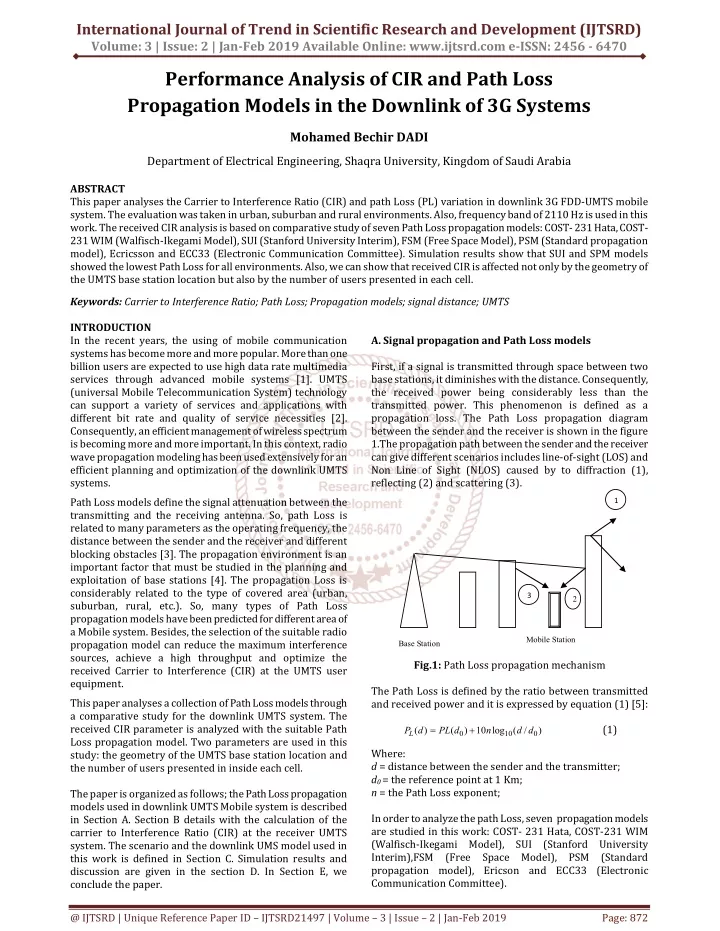
This paper analyses the Carrier to Interference Ratio CIR and path Loss PL variation in downlink 3G FDD UMTS mobile system. The evaluation was taken in urban, suburban and rural environments. Also, frequency band of 2110 Hz is used in this work. The received CIR analysis is based on comparative study of seven Path Loss propagation models COST 231 Hata, COST 231 WIM Walfisch Ikegami Model , SUI Stanford University Interim , FSM Free Space Model , PSM Standard propagation model , Ecricsson and ECC33 Electronic Communication Committee . Simulation results show that SUI and SPM models showed the lowest Path Loss for all environments. Also, we can show that received CIR is affected not only by the geometry of the UMTS base station location but also by the number of users presented in each cell. Mohamed Bechir DADI "Performance Analysis of CIR and Path Loss Propagation Models in the Downlink of 3G Systems" Published in International Journal of Trend in Scientific Research and Development (ijtsrd), ISSN: 2456-6470, Volume-3 | Issue-2 , February 2019, URL: https://www.ijtsrd.com/papers/ijtsrd21497.pdf Paper URL: https://www.ijtsrd.com/engineering/electronics-and-communication-engineering/21497/performance-analysis-of-cir-and-path-loss-propagation-models-in-the-downlink-of-3g-systems/mohamed-bechir-dadi<br>

E N D
International Journal of Trend in Scientific Research and Development (IJTSRD) Volume: 3 | Issue: 2 | Jan-Feb 2019 Available Online: www.ijtsrd.com e-ISSN: 2456 - 6470 Performance Analysis of CIR and Path Loss Propagation Models in the Downlink of 3G Systems Mohamed Bechir DADI Department of Electrical Engineering, Shaqra University, Kingdom of Saudi Arabia ABSTRACT This paper analyses the Carrier to Interference Ratio (CIR) and path Loss (PL) variation in downlink 3G FDD-UMTS mobile system. The evaluation was taken in urban, suburban and rural environments. Also, frequency band of 2110 Hz is used in this work. The received CIR analysis is based on comparative study of seven Path Loss propagation models: COST- 231 Hata, COST- 231 WIM (Walfisch-Ikegami Model), SUI (Stanford University Interim), FSM (Free Space Model), PSM (Standard propagation model), Ecricsson and ECC33 (Electronic Communication Committee). Simulation results show that SUI and SPM models showed the lowest Path Loss for all environments. Also, we can show that received CIR is affected not only by the geometry of the UMTS base station location but also by the number of users presented in each cell. Keywords: Carrier to Interference Ratio; Path Loss; Propagation models; signal distance; UMTS INTRODUCTION In the recent years, the using of mobile communication systems has become more and more popular. More than one billion users are expected to use high data rate multimedia services through advanced mobile systems [1]. UMTS (universal Mobile Telecommunication System) technology can support a variety of services and applications with different bit rate and quality of service necessities [2]. Consequently, an efficient management of wireless spectrum is becoming more and more important. In this context, radio wave propagation modeling has been used extensively for an efficient planning and optimization of the downlink UMTS systems. Path Loss models define the signal attenuation between the transmitting and the receiving antenna. So, path Loss is related to many parameters as the operating frequency, the distance between the sender and the receiver and different blocking obstacles [3]. The propagation environment is an important factor that must be studied in the planning and exploitation of base stations [4]. The propagation Loss is considerably related to the type of covered area (urban, suburban, rural, etc.). So, many types of Path Loss propagation models have been predicted for different area of a Mobile system. Besides, the selection of the suitable radio propagation model can reduce the maximum interference sources, achieve a high throughput and optimize the received Carrier to Interference (CIR) at the UMTS user equipment. This paper analyses a collection of Path Loss models through a comparative study for the downlink UMTS system. The received CIR parameter is analyzed with the suitable Path Loss propagation model. Two parameters are used in this study: the geometry of the UMTS base station location and the number of users presented in inside each cell. The paper is organized as follows; the Path Loss propagation models used in downlink UMTS Mobile system is described in Section A. Section B details with the calculation of the carrier to Interference Ratio (CIR) at the receiver UMTS system. The scenario and the downlink UMS model used in this work is defined in Section C. Simulation results and discussion are given in the section D. In Section E, we conclude the paper. A. Signal propagation and Path Loss models First, if a signal is transmitted through space between two base stations, it diminishes with the distance. Consequently, the received power being considerably less than the transmitted power. This phenomenon is defined as a propagation loss. The Path Loss propagation diagram between the sender and the receiver is shown in the figure 1.The propagation path between the sender and the receiver can give different scenarios includes line-of-sight (LOS) and Non Line of Sight (NLOS) caused by to diffraction (1), reflecting (2) and scattering (3). 1 3 2 Mobile Station Base Station Fig.1: Path Loss propagation mechanism The Path Loss is defined by the ratio between transmitted and received power and it is expressed by equation (1) [5]: log 10 ) ( ) ( 10 0 n d PL d PL Where: d = distance between the sender and the transmitter; d0 = the reference point at 1 Km; n = the Path Loss exponent; In order to analyze the path Loss, seven propagation models are studied in this work: COST- 231 Hata, COST-231 WIM (Walfisch-Ikegami Model), SUI (Stanford University Interim),FSM (Free Space Model), PSM (Standard propagation model), Ericson and ECC33 (Electronic Communication Committee). (1) ( d / d ) 0 @ IJTSRD | Unique Reference Paper ID – IJTSRD21497 | Volume – 3 | Issue – 2 | Jan-Feb 2019 Page: 872
International Journal of Trend in Scientific Research and Development (IJTSRD) @ www.ijtsrd.com eISSN: 2456-6470 Cost-231 HATA Model The Cost 231 Hata model was designed for use in the frequency band of 1500 MHz to 2000 MHz. Although, UMTS downlink band is between 2110 MHz and 2200 MHz. So, it can be assumed, that the model is also valid in this downlink band after tuning [6] [7]. The base station height ‘hb ‘ range is (30 m – 200 m); The receiver antenna height ‘hm ‘is (1m- 10 m); The distance between two antennas ‘d ‘ is from 1km - 2 km. The path Loss PL in dB is equal to [7]: C d B A d PL ) ( log ) ( 10 (2) Where: 82 . 13 ) ( log 9 . 33 3 . 46 10 c f A ) ( log 55 . 6 9 . 44 10 b h B fc is the carrier frequency in MHz Cm= 0 for urban and suburban areas; = 3 dB for rural area; a(hm) is defined for urban environment as: . 4 )) 75 . 11 ( (log 320 ) ( 10 m h a For suburban and rural environments, a(hm) is equal to: 56 . 1 ) 7 . 0 ) ( log . 1 . 1 ( ) ( 10 m m h f h a Cost-231 WIM Model This propagation model describes various areas with different parameters. The cost-231 model has two separate equations for NLOS and LOS line [8]. For Urban environment, the path loss is expressed as [9]: msd rts FSL L L L d PL ) ( (7) Where: 20 ) ( log 20 45 . 32 10 FSL d L f w L ) ( log 10 ) ( log 10 9 . 16 10 10 Where: 35 ) 35 ( 075 . 0 5 . 2 ori L ) 55 ( 114 . 0 4 ori L ) 35 ( 075 . 0 5 . 2 ori L ( log 20 ) ( log 20 10 10 c e msd f d k L For suburban environment, the path loss is given by [9]: L L L d PL ) ( With 1 ) 925 / ( 5 . 1 4 f kf For Rural environment, the path loss is equal to: log 20 ) ( log 26 6 . 42 ) ( 10 10 d d PL SUI (Stanford University Interim) Propagation Model The propagation model is derived from the HATA model with frequency greater than 1900 MHz. The transmitter antenna height is between 10 m and 80 m and the receiver antenna height is between 2m and 10m. The model defines three terrain categories of terrain, namely A, B and C. The path Loss propagation model is given by [10]: X d d A d PL ) / ( log 10 ) ( 0 10 ) / 4 ( log 20 0 10 d A h c bh a / Where: Xf : The correction for frequency in MHz Xh : The correction for receiving the antenna height in meters S: The correction for shadowing in dB; : The path loss exponent; d0=100 m; a, b and c are constants and they are related to the type of the terrain as defined in the table 1. Table 1: SUI Model terrain parameters Parameters Terrain A Terrain B Terrain C a 4.6 b 0.0075 c 126 FSM (Free Space Model) The propagation environment for this model is assumed as a free space and there are no obstacles in the alleyway between the transmitter and receiver. Free Space Model is various on frequency and distance and the Path Loss equation is defined as [11]: d ( log . ) d ( PL 10 20 45 32 SPM (Standard Propagation Model) The standard propagation model is derived from the formula Hata. It is suitable for frequencies between 150 MHz and 3500 MHz and for long distance between 1 km and 20 km. The Path Loss equation in dB in equal to [12]: A f A A d PL ) ( ) ( log . 10 Where: A1, A2, A3, B1, B2, and B3: Hata parameters hb defines the transmitter antenna height; Cclusteris the cluster correction function; hm is the receiver antenna height; d is the distance in km; fc is the carrier frequency in MHz. The Hata parameters of different terrain for SPM models are detailed in the table 2. Table 2: Hata Parameters of SPM model Parameters Urban A1 24,45 A2 44,900002 44,900002 44,900002 A3 5,83 B1 0 B2 -6,55 B3 0 Ccluster 0 Ericsson Propagation Model This model is an extension of Okumara hata Model. It is used for three environments such as urban, suburban and rural. The path Loss equation of the Ericson model is done by [13]: ( log ) ( log ) ( 10 2 10 1 0 f g h Where [log 78 . 4 ) ( log 49 . 44 ) ( c f f g 4 3.6 0.005 20 0.0065 17.1 m (3) (4) log ( h ) a ( h ) 10 b m (18) ) 20 log ( f ) 2 (5) 10 c 97 (6) 8 . 0 log ( f ) 10 c ( ) log ( ) log ( h ) [ B B og ( h ) B h ] 1 2 10 c 3 10 b 1 2 b 3 b d a h C (19) m cluster (8) (9) log ( f ) 10 c 20 log ( H ) L rts 10 mobile ori (10) 55 55 9 35 0 0 (11) ) Suburban 16,45 Rural 9,45 (12) (13) FSL rts msd 5,83 0 -6,55 0 0 5,83 0 -6,55 0 0 (14) ( f ) PL d a a d a h ) a Log ( h ). log ( d ) b 3 10 b 10 (20) 2 3.2. [log 11 ( . 75 ) ] ( ) 10 m c (15) (16) (17) X S f h 2 (21) ( f )] 10 10 c b b @ IJTSRD | Unique Reference Paper ID – IJTSRD21497 | Volume – 3 | Issue – 2 | Jan-Feb 2019 Page: 873
International Journal of Trend in Scientific Research and Development (IJTSRD) @ www.ijtsrd.com eISSN: 2456-6470 hb defines the transmitter antenna height; hm define the receiver antenna height; fcis the carrier frequency in MHz ; d is the distance in km; In our present work, we will study the downlink UMTS –FDD system (base station sends and mobile station receives) as described in the figure 2. Then, the source of interference will be the other base stations that transmit on the same frequency and the radio signal of which will be received by the studied mobile station. Table3. Default values of Parameters in Ericson Model Environment a0 Urban 36.20 30.20 -12.0 0.1 Suburban 43.20 68.90 Rural 45.95 100.6 The different parameters (a0, a1, a2, a3) for various type of terrain are given in table 3. ECC33 (Electronic Communication Committee) Model The ECC-33 propagation model is used for the high frequencies. The path Loss equation for the ECC-33 model is defined as [14]: G G A A PL Where: Afsis the free space attenuation; Ahmis the basic median Path Loss; Gb is the base station height gain; Gr is the received antenna height gain. Then, Afs , Ahm , Gband Grare, respectively, defined as: log 20 ) ( log 20 4 . 92 10 fs d A a1 a2 a3 12.0 12.0 0.1 0.1 Fig.2: Intra and Inter cell interferences The total interference I is composed by two parts: intra-cell interference and inter-cell interference is caused the partial loss of orthogonality interference. Intra-cell (22) between the different codes attributed by the Base station to all users in the same cell. However, the interference inter-cell that is the power received by mobile station from Base station in adjacent cells. The mathematical model to calculate the intra-cell interference on mobile station, MSi served by the base station, BSj is given by [15]: DL i ra P P I , , , int ( Where: Ptotal,jis the total power transmitted by the base station BSj; Pj,iis the the transmitted power from BSj to MSi, α the orthoganality factor and PLi,j define the Path Loss between the MSi and the BSj; fs hm b r (28) (23) (24) ). PL . ( f ) total j j i i , j 10 c 2 A 20 41 . . 9 83 log ( d ) . 7 89 log ( f ) . 9 56 [log ( f )] bm 10 10 c 10 c 2 (25) 8 . 5 G log ( h / 200 )[ 13 958 . [log ( d )] b 10 b 10 For medium city,Gr is equal to: 13 57 . 42 [ r G (26) 7 . log ( f )][log ( h ) . 0 585 ] 10 c 10 m Assuming that the transmitted power by the base station BSj to the each mobile station k, MSk, placed in the same cell of MSi are equals to Pj,i. Then, we can write equation (28) as: N DL i ra N P PL I , 1 Where: Pj,kis the power transmitted by BSj to each mobile station MSk; Nk is the number of mobile station MSk. The mathematical model of the inter-cell interference on mobile station, MSi served by the base station, BSj, is given by: N DL i er P I Where: Ns is the number of all adjacent cell j served by base station BSj; Ptotal,jis the power transmitted by BSj to mobile stationMSi; PLi,j defines the Path Loss between the MSi and the each base station BSj. Assuming that all users have the same bit rate and all base stations BSj transmit the same power Ptotal,jto the mobile station), then: N P P s total , 1 , .... 2 , Then, using equations (30)-(31), we have: And For large city Gr is defined as: 5682 . 1 759 . 0 m r h G Where: hb defines the transmitter antenna height; hm defines the receiver antenna height; fcis the carrier frequency in MHz; d is the distance in km. A.CIR and Path Loss propagation The Carrier To Interference Ratio, CIR, is the most important parameter to evaluate the performance of mobile communication systems. A sufficient CIR must be guaranteed at the receiver in order to diminish the signal attenuation that occurs with radio propagation. CIR is defined as the ratio between the received wanted carrier signal power and the sum of all received interference power. The CIR is calculated as: C I (27) k (29) ) 1 . . ( PL . . P int , i , j j , k k i , j i j , k k i s (30) ( P ). PL ) int , total , j i j , i , j j 1 C (28) CIR n I P n N Where: C is the carrier power happening in the Mobile receiver; I is the total interference In that takes place in the receiver from others base stations; PN represents the total thermal noise power in the receiver and n is the number of interfering base stations. (31) P . total P total N k j , i @ IJTSRD | Unique Reference Paper ID – IJTSRD21497 | Volume – 3 | Issue – 2 | Jan-Feb 2019 Page: 874
International Journal of Trend in Scientific Research and Development (IJTSRD) @ www.ijtsrd.com eISSN: 2456-6470 Where: R is the radius of each cell; is the angle between axis formed by BSj and BSj with MSi. C.Simulation results and discussion The measured data was taken in urban, suburban and rural environments at 2100 MHz all propagation models are calculated using MATLAB Software. Figures 5-7 shows the variation in path loss with the distance d respectively for Urban, suburban and rural areas. All studied propagation models are simulated. So, by observing the path loss variation for urban area in figure 5, it is clear that SPM propagation model have the least path loss and ECC33 propagation model have the highest value in different distances compared with all others propagation models. N s DL ) 1 I ( N ( P . PL ) int er , i k i j , i , j j 1 The final expression of C/I using (28)-(31) is equal to: C CIR P (32) i j , N I s [( N ) 1 . PL . P ] ( N ) 1 ( P . PL ) P k i , j i j , k i j , i , j N j 1 It is clear that the CIR at the mobile receiver is inversely proportional to the path Loss. B.Downlink UMTS model In this paper, the study should focus on the downlink UMTS/FDD system with multi-cell environment. The present model is shown in figure 3. Simulation parameters used in this scenario are given in table 4. Fig.3: Proposed FDD/UMTS scenario Fig.5: Comparison of path loss model variation from urban area Table 1: FDD/UMTS model parameters Parameter Cell number Ns Mobiles number Nk BS Transmission Power [dBm] Frequency Band [MHz] Noise Figure [dB] Orthogonality factor, α chip rate Cell radius, R Processing gain Figure 6 shows the variation of path loss for suburban location. It is clear that SPM model provides the better prediction across all distances compared with others propagation model. However, Value 6 30 43 2110 9 0.7 3.84 Mcps 20 Km 25 In order to calculate the distance between the mobile and each base station, we use the model in figure 4 to simplify the calculation: Fig.6: Comparison of Path Loss model variation from suburban area The simulation results of reviewed models for rural environments are shown in figure 7. IT can be observed that SPM model in rural have the smallest path loss at the same distance compared with results obtained in urban and suburban area. Fig.4: Modeling of distance between Mobile and base station Where dj is the distance between MSi and the suitable base station BSj. dk define the distance between MSi and other base station BSk.Using the formula of EL Kashi [16], we can write: 2 2 (33) d d ( 3 R ) 2 3 R cos i k @ IJTSRD | Unique Reference Paper ID – IJTSRD21497 | Volume – 3 | Issue – 2 | Jan-Feb 2019 Page: 875
International Journal of Trend in Scientific Research and Development (IJTSRD) @ www.ijtsrd.com eISSN: 2456-6470 Fig.9: CIR variation with the number of user. If we increase the number of user in the same cell, the total interference will be increase. Consequently, the CIR at received system is inversely proportional to the number of user. The interference level is directly related to the user’s density in the same cell. D.Conclusion The main objective of this research is to analyze the path loss propagation models and CIR effects for urban, suburban and rural environments in FDD/UMTS system. The path loss has been simulated using seven models, COST- 231 Hata, COST- 231 WIM (Walfisch-Ikegami Model), SUI (Stanford University Interim),FSM (Free Space Model), PSM (Standard propagation model), Ericson and ECC33 (Electronic Communication Committee) models. Path loss values of different models are analyzed and compared in urban, suburban and rural environments at 2110 MHz It can be concluded that SPM model gives better results for all environments. The CIR calculation and simulation with SPM model is detailed for a FDD/UMTS scenario. Simulation results show that the CIR at received system is inversely proportional to the number of user in the cell and it is affected by the position of mobile. Fig.7: Comparison of path loss model variation from rural area The SPM model is used in figure 8 in order to simulate the variation of CIR with distance for different angles . It can be observed that the With the smallest distance d, the variation of angle has not effect on the CIR at received signal; however, for long distance, a small angle can increase the interference and will degrade CIR. The best CIR value is taken with an angle of 120° in this case. Figure 9 shows the variation of CIR with the number of user in the same cell. An angle of 120° has been chosen for this simulation The SPM model is used in figure 8 in order to simulate the variation of Fig.8: CIR variation with angle for different distances References [1]Harri Homa and Antti Toskala, “WCDMA for UMTS—Radio Access for Third Generation Mobile Communications,” Wiley, Chichester, 1st edition, 2000. [2]Suresh Kumar et al, “Quality of service in UMTS networks”: Bell Labs technical journal, Vo. 7, issue 2, 2017. [3]Boulmalf, M., Aouam, T., Harroud, H., “Dynamic Channel assignment in IEEE 802.11 Networks,” International Journal of computer applications.Vo.149. NO.1, 2016. [4]Laiho, J., Wacker, A., Novosad, T., “Radio Network Planning and Optimization for UMT,” Wiley, New York. 2002. [5]M. A. Masud, M. Samsuzzaman & M. A. & M. A. Rahman, ,“ Bit Error Rate Performance Analysis on Modulation Techniques of Wideband Code Division Multiple Access”, Journal Of Telecommunication, Volume 1, Issue 2, PP. 22-29, March 2010 [6]A. Neskovic, N. Neskovic & G. “Paunovic, Modern approaches in modeling of mobile radio system propagation environment“, IEEE Communications Surveys· 2000 @ IJTSRD | Unique Reference Paper ID – IJTSRD21497 | Volume – 3 | Issue – 2 | Jan-Feb 2019 Page: 876
International Journal of Trend in Scientific Research and Development (IJTSRD) @ www.ijtsrd.com eISSN: 2456-6470 [7]Z. Nadir & M. Idrees Ahmad,” Path loss Determination Using Okumura-Hata Model and Cubic Regression for Missing Data for Oman”, Proceeding of IMECS, Vol. 2, 2010. [8]Damosso, E. and Correia, L. M,” Digital Mobile Radio Towards FutureGeneration Systems”, COST 231 Final Report, Brussels, Belgium, 1999 [9]S. Chowdhurz and S. Alam, “Performance evaluation of different frequency bands of WiMAX and their selection procedure”, IJAST journal Vo. 62, N0.01, pp 1-18. [10]Erceg, V., K. Hari, M.S. Smith and D.S. Baum,” Channel models for fixed wireless applications”, IEEE Tech. Report .2001. [11]V. S. Abhayawardhana, I. J. Wassel, D. Crosby, M.P. Sellers, and M.G., Brown,” Comparison of empirical propagation path loss models for fixed wireless access systems”, 61th IEEE Technology Conference, Stockholm. 2005. [12]Rani, M. Suneetha, Subrahmanyam VVRK Behara, and K. Suresh,” Comparison of Standard Propagation Model (SPM) and Stanford University Interim (SUI) Radio Propagation Models for Long Term Evolution (LTE)”, IJAIR Journal, 2012. [13]J. Milanovic, S. Rimac-Drlje, and K. Bejuk,” Comparison of propagation models accuracy for WiMAX on 3.5 GHz” 14th IEEE International Conference on in Electronics, Circuits and Systems, 2007. pp. 111-114 [14]P. K. Sharma and R. K. Singh, “Comparative Analysis of Propagation Path Loss Models with Field Measured Data,” Int. J.Eng. Sci. Technol., vol. 2, no. 6, pp. 2008–2013, 2010. [15]Sugano, M., Kou, L., Yamamoto, T. and Murata, M., “Impact ofSoft Handoff on TCP Throughput over CDMA WirelessCellular Networks”, in Proc. of VTC 2003 Fall – IEEEVehicular Technology Conference, Orlando, FL, USA @ IJTSRD | Unique Reference Paper ID – IJTSRD21497 | Volume – 3 | Issue – 2 | Jan-Feb 2019 Page: 877