Download
1 / 81
840 likes | 1.34k Views
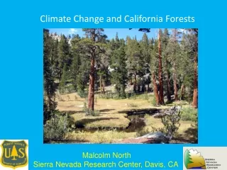
Climate Change and California. Michael Hanemann Dept. Agricultural & Resource Economics, UC Berkeley. Topics. Climate Change is Happening The Contrast between Europe and the US Climate Change and California Climate Change Impacts Climate Change Policy.

E N D
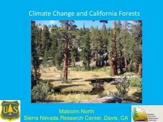
Climate Change and California Michael Hanemann Dept. Agricultural & Resource Economics, UC Berkeley
Topics • Climate Change is Happening • The Contrast between Europe and the US • Climate Change and California • Climate Change Impacts • Climate Change Policy
A warming Northern Hemisphere –the famous hockey stick • IPCC - 2001
More than 30% increase in atmospheric CO2 since thebeginning of the industrial revolution
Climate Change 1. Climate change is happening already. There is considerable evidence of change. • The global average temperature was increasing by about 1/10 degree F every decade until about 1970, but has been increasing about 5/10 degree F per decade since then. • Since about 1950 snow accumulation has already shown losses on the order of 10% in April 1 snow water equivalent across the western United States (Mote et al. 2005). • Over this period, the onset of the snowmelt spring pulse has shifted earlier in time by 10–30 days throughout the western United States (Stewart et al. 2005). • In California, the 100-year, 3-day peak flows on the American, Tuolumne, and Eel Rivers have more than doubled between the first and second halves of the twentieth century (Chung, 2005).
Responses to earlier springs • Average advance in signs of spring: 2.3 days/decade • Budburst, flowering, nesting, fledging, etc. • 172 species (trees, shrubs, herbs, butterflies, birds, amphibians, fish • Parmesan & Yohe 2003 Nature v 421 p 37 • Advancing bud-burst date: • 2.5 days/decade • 1900-1998 • Aspen in Edmonton • Beaubien & Freedland. 2000. Int J. Meteorol.
Altered range limits • Average change in “cold” limit:4 miles/decade North or 20’ higher/decade • 99 species (plants, birds, & butterflies) • 81% of range changes in expected direction • 372 species (trees, shrubs, herbs, birds, mammals, reptiles, amphibians, fish, insects, & marine invertebrates) • Parmesan & Yohe. 2003. Nature
Wildfire and warming Gillett et al. 2004. Geophys. Res. Lett.
Trends in US agriculture • Over the last 50 years, yields of US corn & soybeans increased 1-2%/year • But year-to-year increases were larger in cooler years and smaller in warmer years • A warming of 1º F decreased yields by 9% • Lobell & Asner. 2003 Science
Conventional view in Washington • The conventional view in DC is that • Climate change poses relatively little risk to the US in the near term, and may even be beneficial • The cost of any large reduction in US emissions would be economically harmful • Hence the notion of setting a modest price of carbon and seeing what happens
Stern Review • Review of economics of climate change commissioned by the Chancellor of the Exchequer, conducted by Sir Nicholas Stern Head of the UK Government Economic Service, released in November 2006. • Calls for “prompt and strong action….If we don’t act, the overall costs and risks of climate change will be equivalent to losing at least 5% of global GDP each year, now and forever.”
Reception of Stern • Nordhaus (2006): The Stern Review results are “dramatically different” from existing economic analyses. • He finds that optimal economic policy for climate change involves modest rates of emissions reductions in the near term. 6% emissions reduction in 2005; 14% in 2050; and 25% in 2100.
Why the different conclusions? • Choice of interest rate used for balancing future damage avoided versus present costs of abatement. • Stern uses a much lower interest rate • Assessment of future damages • Stern’s assessment of these is much greater • Uncertainty and risk aversion factored in by Stern but not Nordhaus • Assessment of costs of emission reduction • Stern’s assessment of these is lower
Sources of climate impact • Change in temperature • Change in precipitation • Change in sea level triggered by change in temperature • These play out differently and on different time scales.
Climate Change & the California Energy Commission • 1991 Funds study of climate change impact on California water. • 1997 Public Interest Energy Research (PIER) Program initiated funded by surcharge on electric bills. • CEC Designated lead state agency on climate change. • 2000-2002 First assessment study of climate change impacts on California • 2003 California Climate Change Center established; second assessment launched
Climate Change as an Issue in California • 2002: AB1493 passed to reduce GHG emissions from motor vehicles in California. • 2003 Fall: Union of Concerned Scientists launches scenarios study, leading to paper in Proceedings of National Academy of Sciences August 2004. • January 2004: Governor Schwarzenegger takes office • September 2004: California Air Resources Board approves regulations to implement AB 1493. • June 2005: Governor Schwarzenegger announces GHG emissions reduction targets for California and calls for report to Legislature by January 2006 on climate change policies and impacts of climate change on California.
California’s 2006 GHG laws • AB 32, places a cap on all GHG emissions in California; requires that, by 2020, these be reduced to their 1990 level, a reduction of ~29%. • SB 1368 Prohibits any load-serving entity from entering into long-term financial commitment for baseload generation unless GHG emissions are less than from new, combined-cycle natural gas. Applies to out-of-state generators, also to municipals.
Other components • AB 1493 Imposes emissions cap on fleet of new model vehicles sold in California. • Enacted 2002; regulations issued 2004 • Near term (2009-2012): 22% reduction in GHG emissions (grams of CO2e/mile) • Mid-term (2013-2016): 30% reduction in GHG emissions • Low Carbon Fuel Standard: ≥ 10% emission reduction by 2020 • CPUC Carbon adder $8/ton • Renewable Portfolio Standard 33% by 2020
Taken together, these are the most ambitious and comprehensive effort to control GHG emissions in force in the US. • They apply: • To all GHGs, not just CO2 (CO2 from fossil fuel combustion is 81% of all GHGs in CA) • To all sources, not just electric power plants (= 22% of all GHG emissions in CA). • The only other binding cap on emissions is RGGI
US Greenhouse Gas Emissions Source: EPA. 2002 Emissions, including CO2, CH4, N2O, HFCs, PFCs, and SF6.
California GHG Sources2002 Emissions Source: CEC. Gross emissions only.
The Scenarios Study of Climate Change Impacts on California • Hayhoe et al., Proceedings of the National Academy of Sciences, August 24, 2004. • Governor’s Report on climate change http://www.climatechange.ca.gov/climate_action_team/reports/index.html
The new impact (“Scenario”) analyses The new analyses contrast two global emission scenarios: (i) business as usual with continuing high rate of growth in greenhouse gas (GHG) emissions; and (ii) sustained global effort to reduce GHG emissions by 2100. The analyses use statistical downscaling to translate the larger scale global climate model results to California with finer resolution (grid scale = 12 km).
Global Climate Models compute Climate on a coarse grid So, a “downscaling” procedure was used to provide temperature and precipitation over a finer mesh that is more commensurate with the California landscape A hydrologic model is used to simulate streamflow, soil moisture and other hydrologic properties
Structure of the Overall Study Global Climate Models Statistical Downscaling and Hydrological Modeling: common set of scenarios Water Costal Impacts Agriculture Forest Sector Public Health Electricity
How are the new versions of these climate models different? • The new versions of both models are somewhat more pessimistic with regard to precipitation than the previous two versions. • The new versions are substantially more pessimistic with regard to the increase in summer-time temperature. • The latter result may be due to improved modeling of the linkage between surface temperature and ambient air temperature.
Temperatures in California are predicted to rise significantly
Time Lags • The temperature trajectories for the two emission scenarios remain fairly intertwined until about 2045. • They illustrate the fact that California’s future climate for next 40 years is already determined by past emissions. • Emission reductions initiated now show a significant effect after about 2045, with their impact increasing over time.
Rising TemperaturesCalifornia statewide Projected average summer temperature changes
18.0 °F 14.4 10.8 7.2 3.6 0.0 -3.6 Patterns of Temperature Change2070-2099 relative to 1961-1990Summer LOWER EMISSIONS HIGHER EMISSIONS PCM lower HadCM3 lower PCM higher HadCM3 higher
Climate Change and Agriculture • The most heavily analyzed sector in climate economics literature. • Also the most divergent range of estimates e.g., from loss of 25% in value of US ag output to gain of 20%.
Interactions between climate & crop growth Complex, non-linear, not unidirectional, and multidimensional: • Temperature • Effects on yield • Effects on quality • CO2 fertilization • Crop ET (crop water need) • Weeds, pests • Ozone
Existing literature focuses just on temperature and CO2 fertilization; focuses on crop yield, not quality, especially major grain crops. • Other effects largely ignored so far. • When attention is thus restricted, estimated, climate change impact on yield can well be positive: • Fertilization effect is positive • Cooler areas benefit from warming
Three factors • Characterization of temperature change • Annual, seasonal, monthly, daily • Global, US, California, Central Valley • Assumed shape of relationship between temperature and yield • Symmetric, hill-shaped • Asymmetric, mesa-shaped • Allowance for economic adaptation
Schlenker & Roberts (2006) Relation of Temperature and Crop Yield • Relationship is not symmetrical; it is distinctly asymmetric, fairly flat at first and then sharply declining beyond an upper threshold.
Economic adaptation • The extent to which a physical change in yield translates into a corresponding change in output supplied depends on • Supply and demand in market for product and in related markets • Other responses and adaptations • Change planting/harvest dates • Change cropping pattern • New seed varieties • Change land use • etc
Two approaches to incorporating adaptation • Combine crop yield model with some model of economic market behavior. • Led to estimates of loss to US agriculture ranging from $1.1 billion to $17.5 billion. • Ricardian Approach (Mendelsohn, Nordhaus and Shaw, 1994) [MNS]. Regress farmland value directly on climate variables. In theory, allows for adaptation to a greater extent. • Gain of $2.5 billion, $24 billion.
The difference was widely attributed to the economic effect of adaptation. • In fact, it arises from some flaws in MNS’s statistical analysis of their data involving their failure to control adequately for irrigation (Schlenker, Hanemann and Fisher 2005). • Irrigation breaks the link between precipitation where crop is grown and the amount of plant growth. • In Iowa, 22” of growing season precip, 100% of crop water need for corn • In California, 1.5” of growing season precip, 5% of crop water need for cotton. • Therefore, need to analyze irrigated areas separately from rainfed areas.
When MNS analysis is repeated just for rain fed areas of US, instead of a gain for these areas of $2.3 billion, there is a loss of $11 billion. • Irrigated areas need individual analysis based on a measure of their water supply; but there clearly is a net loss: • Increased crop demand for water • Reduced supply of water • There is no evidence that, when correctly implemented, Ricardian approach yields substantially different estimates of loss from models of agricultural market models.
Adaptation • Adaptation will clearly occur and will mitigate loss. • But adaptation will not occur instantaneously, will not be costless, and may not be perfect. Thus there are losses associated with adaptation. • None of the existing economic analyses accounts for this.
Importance of spatial and temporal details for water supply • 2/3 of precipitation occurs north of Sacramento. • About 2/3 of all water use occurs south of Sacramento. • 80% of precipitation occurs October-March. • 75% of all water use occurs April – September. • Snow pack holds the equivalent of ~1/3 of our major storage capacity