Download
1 / 72
730 likes | 837 Views
Pacific Subtropical Highs: Features Interacting with Midlatitude and Tropical Forcing. Richard Grotjahn Atmospheric Science Program, Dept. of LAWR, Univ. of California Davis, CA 95616, USA. Organization of this talk:. Some Simple Observed Facts Some simple conceptual models and questions

E N D
Pacific Subtropical Highs: Features Interacting with Midlatitude and Tropical Forcing Richard Grotjahn Atmospheric Science Program, Dept. of LAWR, Univ. of California Davis, CA 95616, USA
Organization of this talk: • Some Simple Observed Facts • Some simple conceptual models and questions • Monthly mean observed data analysis • Daily observed data analysis • Summary
A Simple Fact about the Subtropical Highs • On a zonal mean, they are strongest in winter.
Pacific Subtropical Highs - Summer • Found on the eastern side of each subtropical ocean (in summer) • North Pacific or “NP” high (JJA) • South Pacific or “SP” high (DJF)
Some Simple Facts about the Pacific Highs • On a long term monthly mean, the central pressure is greatest in a season OTHER than winter. • Summer (North Pacific) • Spring (South Pacific)
Subtropical Highs Seasonal Variation • In N. Hemis: • The peak value is greater for N. Atlantic and NP highs during summer. • But, the zonal mean includes lower than annual average pressure over land areas in summer. • In winter SLP pattern is more uniform with longitude, making the zonal mean greatest in winter • In S. Hemis: • SP high similar in winter and summer. Strongest in spring. • S. Atlantic and S. Indian highs stronger in winter than summer. Grotjahn, 2003
Test: In what month did this day occur? • The point? • This “summer” pattern reflects an absence of frontal cyclone activity. • Frontal cyclones obscure our perception of the subtropical high strength. • Perhaps they contribute to the high. • July? • August? • June? The actual date is: 15 January 2000 Image provided by the NOAA-CIRES Climate Diagnostics Center, Boulder, Colorado, from their Web site at http://www.cdc.noaa.gov/.
Planet: Aqua • Uniform surface, uniform “Hadley” cell. • N. Hemisphere summer
Planet: Aqua-terra • Now include land areas (summer) • Land areas hotter than cooler ocean areas
Planet: Aqua-terra 2 • Now allow subsidence over W land areas: extra solar heating & adiabatic compression • Equatorward motion causes ocean upwelling
Simplified “PV” analysis • Surface cold area: anticyclonic PV. So, subtropical high (H) over ocean. • Surface warm area: cyclonic PV. So, thermal low over land • Equatorward motion enhances the upwelling, etc. H L
What’s Missing? • interaction with mid-latitudes • connecting the circulation pieces • other forcing mechanisms
The mid-latitude connection • Consider upper level divergent motions.(July) • Va ~ Vdiv • Simplified time mean balance: u du/ dx = f va • (Namas & Clapp, 1949; Blackmon et al, 1977) • Upper level convergence (schematic diagram) • “Hadley” cell extension (red arrows) • Observed pattern less clear. • Atlantic perhaps most like the schematic • Pacific less so Nakamura and Miyasaka (2004) – July conditions 200 mb isotachs (solid); SLP (dashed); meridional ageostrophic wind (arrows)
The mid-latitude connection • Simplified time mean balance: u du/ dx = f va • (Namias & Clapp, 1949; Blackmon et al, 1977) • Upper level convergence (schematic diagram) from equatorward flow: • Northerlies like “local Ferrel cell” with presumably similar forcing: frontal cyclones. Nakamura and Miyasaka (2004) 200 mb isotachs (solid); SLP (dashed); meridional ageostrophic wind (arrows)
Various proposed forcing mechanisms Remote: • subtropical high is element of “Hadley” circulation driven by ICZ • monsoonal circulations to the west (e.g. “Walker” cell; Chen etal) • monsoonal circulations to the east (“Gill” model sol’n; Hoskins etal) • convection spreads to west subtropical ocean from destabilization by poleward motions & ocean circulation (Seager etal) • topographic forcing (planetary wave problem) • non-latent diabatic heating to the east (E sea /W land has large T gradient; Nakamura, Wu, Liu, etc) • midlatitude frontal cyclones (K-E eqn, jet dyn, CAA, merging, etc.) Local: • net radiative cooling (top of stratus deck) • subsidence to east creates equatorward wind (dw/dz ~ bv) • ocean upwelling of cold water (& transport away) • evaporative cooling of eastern subtrop. SST from subsiding dry air (Seager etal)
Divergent Circulations: SP high 100 W • 22-yr mean January meridional cross section • “Hadley” suppressed by “Walker” cell. • Divergent flow from higher latitudes, too. • Sinking equatorward of the high center H
Divergent Circulations: SP high 20 S • 22-yr mean January zonal cross sections • “Walker” cell • Divergent flow from higher latitudes • Sinking stronger to east & poleward 40 S H
Analysis Procedures (Monthly Data) • Preliminary study to identify coincident behavior. • Monthly NCEP/NCAR Reanalysis data (1979-97). • Seasonal groupings, local “summer” emphasized. • Total and monthly anomaly (MA) fields. (MA defined as deviations from the average constructed from all occurrences of that month). • Monthly data cannot distinguish cause from effect. • Tools (significance test) shown here: composites (bootstrap resampling) 1-point rank correlations (t- and D-statistics).
E and NE: lower SLP (purple) more P (N of South America) for strong high and vice versa. N and NW: More P and Northward shift of ICZ W: More P (green) & westward shift of SPCZ NW & N MJO? ENSO? S and SW: Dipole (P) storm track shift to S for strong SP high. Tracks may be broader for weak SP high. NP high: similar results 6 strongest – 6 weakest Blue: significant above (1%) Red: significant below (1%) SP High Composite: ONDJF Monthly Anomaly Data: SLP P - precipitation
Shaded: 2 signif. tests passed; ~0.3 correl. correl. points respond to events on same side: NE to E side: Pacific ICZ shifts away from high & more Amazonian P NW side: to ICZ & SPCZ shift away from high E, NE, N, and NW sides: correl. w/ less P in the Kiribati area like composites. W, SW & S sides: Total and MA data both show: dipolar pattern => poleward shift of storm track for higher SLP Composites consistent P shown, OLR similar Blue: significant below (1%) Red: significant above (1%) 1-pt correlations of Monthly Anomaly Data:
Signif. R at remote spots on the same side of the high as the correl. point. P near Central America not compelling. For key points on the East side of the high, less P for stronger SLP. Results consistent w/ composites* P shown, OLR similar Blue: significantly (2.5%) more P for higher SLP at * Brown: significantly (2.5%) less P for higher SLP at * H is total data mean location 1-pt correlations of MA Data: NP High
Data Source: NOAA/CDC (Boulder CO, USA) NCEP/NCAR reanalysis data SLP, U, V Ud, Vd, Velocity Potential (VP) from NCL commands. Data record: 90-day DJF periods shown (122 day NDJF similar) Drawn from 01/1990 through 08/2002 Goal: Prior work showed remote links now wish to establish cause and effect by using lags and leads. Work with Daily Mean Data: SP high only
Velocity Potential (“VP”) at 200 hPa lag (L) and lead (R) SLP @ pt-8 correl: (CW: 8, 6, 4, 2, 0, -2, -4,-6 d) Red: >0 Blue: <0
Observed Divergent Wind Field • SP high • NP high
Vd – Meridional Divergent Windat 200 hPa & SLP @ pt-11 correlations (CW: 4, 2, 0, -2, -4d)NP high: similar pattern
What about the NP high daily data? • NP high very strongly influenced by day to day variation associated with traveling frontal cyclones. • NP high more strongly varies than SP high, which suggests filtering and/or subsampling to remove the high frequency variation from frontal cyclones.
Sub-sampled SLPda-OLRda Filter or not? SLP 8 days after OLR Raw SLPda-OLRda Filtered and sub-sampled SLPda-OLRda
Midlatitude Cyclone Interaction Example • Motions relative to upper level ridge in central N. Pacific. Summer climatology has ridge along N. America west coast • Sinking SE of upper level ridge. Fig. 24: Lim & Wallace (1991) • Divergent wind fields as deduced from 1-pt (using F500) correlations with constant Coriolis basis ageostrophic wind. Fig 14: Lim et al. (1991) • Higher SLP at mean NP high loc. w/ similar Udiv, Vdiv upper level convergence NE of the NP high center. SLP-Vdiv SLP-Udiv 0 lag
NP high: Meridional divergent wind (da) • Filtered & Subsampled 8, 4, 0, 4 d lags Red: > 0 Blue: < 0
Composites: NP high SLP (da): JJA • Strong highs • Weak highs • Strong-weak • Couplet at 0 lag
Surface q – SLP 1-pt correlations: NP high • Point near center of high: 8, 4, 0, -4 d lag. Correlated with cold at high • Near center of high, SLP is followed by high q over southeastern US.
Summary: Observational Results • Each side of each high linked to remote event on same side • Both highs show links to lower and higher latitude events • Stronger highs poleward and W of mean position • Stronger SLP when storm track shifted to higher latitude • Need low pass filter to see NP high links to low latitude events • East side of NP high associated with suppressed Central American P • E side of SP high stronger after enhanced Amazonian P & convection. More so when E. Indonesia convection weakened Conclusions • Evidence of midlatitude (frontal cyclone) forcing; • Mixed evidence for: Direct Cells; Rossby wave upstream; surface temperature forcing (other mechanisms untested)
Question 1 • What observational variable is best for looking at the surface temperature anomaly (forcing a PV anomaly) connection? Tsfc -temperature qsfc –potential temperature Image provided by the NOAA-CIRES Climate Diagnostics Center, Boulder, Colorado, from their Web site at http://www.cdc.noaa.gov/.
Question 2: NP high: Meridional divergent wind (da) Why this correlation? Why precede SLP? • Filtered & Subsampled • 8, 4, 0, 4 d lags • Red: > 0 • Blue: < 0
The End • Acknowledgements: • M. Osman • S. Immel • NSF
Storage • Not used due to time available
Surface q – SLP 1-pt correlations: NP high • Point on S side: 8, 4, 0, -4 d lag. Correlated with cold at the high • On S side, higher SLP led by correlated with high q over PNG.
Forms of diabatic heating • Liu et al (2004)
Focus on 3 remote sources Some connections will be visible through the divergent circulations. P or OLR are proxy for rising motion. Simplest tests: is SLP linked to P in target regions? P intensity? P shifts? P timing? If viewed as planetary wave problem, then topography also has role (1) Hadley and Walker circulations, (2) Rossby wave forcing from East, b v = f dw/dz (3) traveling frontal cyclones and anticyclones Remote Forcing Mechanisms – SP high
Test Proxies of strength of the rising sector of a circulation • P or OLR are proxy for rising motion. • Is SLP linked to: • P in target regions? • P intensity? • P shifts? • P timing? • Other scalar parts of divergent circulation? • Velocity potential • Divergent wind components, speed
NP high Composite: JJA Monthly Anomaly Data: • 6 strongest – 6 weakest • Green: significant above (1%) • Purple: significant below (1%) • SLP: • Highest when high is NW • SP high coordinated • Weak & strong composites not “opposite” • Precip: • Shift of ICZ southward • Shift of midlat NW-ward • Stronger over Indonesia
Velocity Potential (“VP”) at 200 hPa lag (L) and lead (R) SLP @ pt-8 correlations (CW: 8, 6, 4, 2, 0, -2, -4,-6 d)