Download
1 / 35
350 likes | 423 Views
Cost and Benefit. Avinash Kishore ( avinash.kishore@gmail.com ) Based on notes from Andrew Foss Economics 1661 / API-135 February 11, 2011 Review Section. Agenda. Basic Econometrics Bi- variate regression Multivariate linear regression Special cases Elasticity Social Welfare Cost

E N D
Cost and Benefit AvinashKishore (avinash.kishore@gmail.com) Based on notes from Andrew Foss Economics 1661 / API-135 February 11, 2011 Review Section
Agenda • Basic Econometrics • Bi-variate regression • Multivariate linear regression • Special cases • Elasticity • Social Welfare Cost • Benefits • Aggregation of Demand Curves • Travelling Cost Method Note: A good general reference on costs and benefits is EPA, Guidelines for Preparing Economic Analyses, September 2000 (link), Chapters 7 and 8
Measures of Central Tendency and Dispersion • Measures of Central Tendency: Mean • Mean = ∑Xi /n • Mean takes all data points into account • Mean is sensitive to outliers. Outliers have a lot of weight on mean • Measures of Dispersion • Variance = (Xi – mean)2/N • Standard Deviation =[(Xi – mu)2/N]1/2 = (Variance)1/2 • More dispersed data have higher variance • Like mean, standard deviation is also sensitive to outliers
It is possible that two datasets have the same mean but different standard deviations From Wikipedia
OLS regression (2 Variables) http://www.ats.ucla.edu/stat/Stata/examples/rwg/rwgstata2/rwgstata2.htm Y (wateruse) = 1201.124 + 47.54*income
Bi-variate Regression Model • Yi = β0 + β1Xi + εi • i = each observation; Y = Dependent Variable (water use); X = Independent Variable (income); εi = Error term • β0 = intercept. It tells us the predicted value of Y when X = 0. • β1 = The coefficient that tells us how Y changes for unit change in X. • water81 Coef. Std. Err. t P>t [95% Conf. Interval] • income 47.54869 4.652286 10.22 0.000 38.40798 56.6894 • _cons 1201.124 123.3245 9.74 0.000 958.8191 1443.43 • N = 496; R-square = 0.1745 • 3 Sources of Error Term: • Omitted variables, Measurement error and Chance or Randomness
Multiple Regression • More than one independent variables • Yi = β0 + β1Xi1 + β2Xi2 + β3Xi3 + εi • Now, β1 is the change in value of Y for a unit change in X1 while holding constant (or controlling for) X2 and X3 (the marginal interpretation) • Example:. reg water81 income educat peop81 • water81 Coef. Std. Err. t P>t [95% Conf. Interval] • income 32.05796 4.285087 7.48 0.000 23.63864 40.47729 • educat -42.61099 17.23512 -2.47 0.014 -76.4745 -8.747484 • peop81 480.5194 31.73071 15.14 0.000 418.175 542.8639 • _cons 678.8889 245.195 2.77 0.006 197.1305 1160.647 N = 496, R-squared = 0.38
Some Special Cases: binary independent variables • Normally, continuous dependent and independent variables in OLS. • But we can also have binary independents. Also Dummy Variables. • Βeta coefficient of a dummy variable is not interpreted as its slope. • Let there be a dummy variable Females.t. Female = 1 for female employees; 0 for male employees. • Regression equation: Earnings = β0 + β1*Female + εi • Earnings = 16.99 – 3.45*Female + εi • Interpretation: Constant, β0 = Mean earning of men = 16.99 β1 = Difference in mean earnings of men and women. Here, β1 = -3.45. So, mean earning of women = 16.99 – 3.45 = 13.44. • Multivariate Example: • Earnings = β0 + β1 Years of Education + β2Female + εi • Earnings = 15.55 + 3.00* Years of Education –3.55*Female • Show graphically
Special Cases: Interaction Terms • It is possible that both intercepts and slopes (returns per year of education in this case) are different for two groups. • e.g. Earnning = β0 + β1Years of Education + β2Female + β3 Female*Years of Education + εi • So, for females: Earnings = β0 + β1Years of Education + β2*1 + β3*1*Years of Education+ εi • = (β0 + β2) + (β1+ β3)*Years of Education+ εi • for males: Earnings = β0 + β1Years of Education + β2*0 + β3*0* Years of Education + εi • = β0 + β1Years of Education + εi • So, for females, Slope = (β1+ β3) and Intercept = β0 + β2 • For males, Slope = β1and intercept = β0
We can also capture non-linear relations through linear regression • Quadratic: If the dependent variable is a parabolic function of the independent, we can still capture the relationship by adding a squared term, e.g. Environmental Kuznets Curve hypothesis: • Pollution = β0 + β1GDPPC + β2 (GDPPC)2 + εi • Categorical Dependent Variable (as in RUM) • We get estimates of probability • OLS is not appropriate in such cases • Logit or probit models
Costs Estimation Methods and Elasticity • Direct Compliance Cost Method • Partial Equilibrium Analysis (behavioral response) • General Equilibrium Analysis • Want to know how consumers and firms will react to changes in prices for the good/service being regulated • Depends on price elasticity of supply and demand • Elasticity = % ΔQ/% ΔP = (ΔQ/Q)/ (ΔP/P) = (ΔQ/ΔP)*(P/Q) = (1/Slope)*(P/Q) • Higher the elasticity, greater the behavioral response to regulation and greater the social welfare cost.
If demand is very responsive to change in price, good is price elastic. If demand does not respond much to price changes, demand is price inelastic Elasticity = ∞ Elasticity = 0
Social Welfare Costs • Illustration of social welfare costs • Losses in consumer and producer surplus from increased marginal cost across regulated industry Welfare Effects of Industry-Wide Increase in Marginal Cost Price Price MC1 = S1 D D CS1 MC0 = S0 MC0 = S0 CS0 P1 P0 P0 PS1 PS0 Quantity Quantity Q0 Q1 Q0
Benefits: Aggregation of Demand Curves (Private Goods) Let’s say Q is a private good. Person 1 demand for Q is: Q1 = 100 – P Person 2 demand for Q is : Q2 = 100 – P So, what is the aggregate market demand for Q? Algebraically, it is QT = 200 – 2P Note: The algebra and the graph won’t be this simple if demand functions are different
Benefits: Aggregation of Demand Curves (Public Goods) Now assume Q is a public good (non-rivalrous and non-excludable) Does that change how we aggregate demand curves? Algebraically, it is P= 200 – 2Q You work with inverse demand curve
One more example: public park provision • There are 500 people in a locality • Each has demand function: Q = 100 – P • P = $ price per unit area of park people are willing to pay for Q sq. yards of the park preserved • MC = $ 10,000/sq. yard • How many sq yard of park area should be preserved? • P = 100 – Q • Aggregate demand: P =500[100 – Q] • or P = 50,000 – 500Q • 50,000 – 500Q = 10,000, Q* = 80 sq. yards • What is the total benefit @ Q*? Net benefit = ?
Travel Cost Method:Example Problem • Ruritania is a country with three cities and a beautiful park at its center • Environmental economists in Ruritania have collected the following data on park visitors from the three cities • The environmental economists want to estimate the recreational value (i.e., non-market use value) of the park to the people of Ruritania
Travel Cost Method:Example Problem • First calculate the visitation rate for each origin
Travel Cost Method:Example Problem • Next plot the relationship between visitation rate and travel cost and express it in an equation TC = - (50 / 0.20) * R + 50 = -250 * R + 50 or R = - (0.20 / 50) * TC + 0.2 = -0.004 * TC + 0.2
Travel Cost Method:Example Problem • Suppose a fee were charged to enter the park • Calculate the relationship between Origin 1’s visitation rate and the hypothetical fee R = -0.004 * (TC + Fee) + 0.2 TC1 = 12.5 R1 = -0.004 * (12.5 + Fee) + 0.2 = -0.004 * Fee + 0.15 or Fee = -250 * R1 + 37.5
Travel Cost Method:Example Problem • Calculate the relationship between Origin 2’s visitation rate and the hypothetical fee R = -0.004 * (TC + Fee) + 0.2 TC2 = 25 R2 = -0.004 * (25 + Fee) + 0.2 = -0.004 * Fee + 0.10 or Fee = -250 * R2 + 25
Travel Cost Method:Example Problem • Calculate the relationship between Origin 3’s visitation rate and the hypothetical fee R = -0.004 * (TC + Fee) + 0.2 TC3 = 37.5 R3 = -0.004 * (37.5 + Fee) + 0.2 = -0.004 * Fee + 0.05 or Fee = -250 * R3 + 12.5
Travel Cost Method:Example Problem • Calculate the relationship between all three origins’ visitation rate and the hypothetical fee R = -0.004 * (TC + Fee) + 0.2 R1 = -0.004 * Fee + 0.15 R2 = -0.004 * Fee + 0.10 R3 = -0.004 * Fee + 0.05
Travel Cost Method:Example Problem • Calculate the relationship between the number of visitors from Origin 1 and the hypothetical fee Per capita demand function: R1 = -0.004 * Fee + 0.15 Population = 100,000 So, demand function is: = 100,000*(-0.004 * Fee + 0.15) = -400 * Fee + 15,000
Travel Cost Method:Example Problem • Calculate the relationship between the number of visitors from Origin 2 and the hypothetical fee Per capita demand function: R1 = -0.004 * Fee + 0.10 Population = 75,000 So, total demand function is: = 75,000*(-0.004 * Fee + 0.10) Q2 = -3,000 * Fee + 75,000
Travel Cost Method:Example Problem • Calculate the relationship between the number of visitors from Origin 3 and the hypothetical fee Per capita demand function: R1 = -0.004 * Fee + 0.05 Population = 50,000 So, total demand is: = 50,000*(-0.004 * Fee + 0.05) Q3 = -4,000 * Fee + 50,000
Travel Cost Method:Example Problem • Aggregate curve (from horizontal summation) represents total recreational demand as a function of hypothetic park fee • 1st kink @ Fee = $25, Qagg = 5000 • 2nd kink @ Fee = $ 12.50, Qagg = 10,000 + 37,500 = 47,500 • X-intercept = 15,000 + 75,000 + 50,000 = 140,000 Q1 = -400 * Fee + 15,000 Q2 = -3,000 * Fee + 75,000 Q3 = -4,000 * Fee + 50,000
Travel Cost Method:Example Problem • Calculate recreational value as area under the aggregate curve • The recreational value of the park is $1,531,250 Area A = ½ * (37.5 - 25) * 5,000 = 31,250 Area B = ½ * (25 - 12.5) * (5,000 + 47,500) = 328,125 Area C = ½ * (12.5 - 0) * (47,500 + 140,000) = 1,171,875 Total Area = 1,531,250
Travel Cost Method:Example Problem • Calculate recreational value as area under each of the origin-specific demand curves (alternative method) • The recreational value of the park is $1,531,250 Area 1 = ½ * 37.5 * 15,000 = 281,250 Area 2 = ½ * 25 * 75,000 = 937,500 Area 3 = ½ * 12.5 * 50,000 = 312,500 Total Area = 1,531,250
Travel Cost Method:Example Problem • Calculate the number of visitors and consumer surplus if no fee were charged to enter the park • Total park visitation is 15,000 + 75,000 + 50,000 = 140,000 • CS is equal to recreational value: $1,531,250
Travel Cost Method:Example Problem • Calculate the number of visitors and consumer surplus if a fee of $20 were charged to enter the park • Total park visitation is 7,000 (Or. 1) + 15,000 (Or. 2) = 22,000 • CS is area below demand curve and above price: $98,750 Area A = ½ * (37.5 - 25) * 5,000 = 31,250 Area D = ½ * (25 - 20) * (5,000 + 22,000) = 67,500 Total Area = 98,750
Benefits: Mid-term 2005 • The City of Miami, Florida proposes to invest in a new water reservoir for its public water system, and estimates its cost. To justify this substantial expenditure of public funds, the Mayor explains that if the new reservoir is not constructed then the next most costly way to increase Miami’s water supply will be to invest in a desalinization plant, which will be even more expensive. Hence, the Mayor explains, the social benefits of building the new reservoir clearly exceed its social costs. There are no environmental or other externalities involved with either alternative. How would you assess this reasoning from an economic perspective? • This is the “avoided cost” method of evaluating benefits.It is incorrect because it ignores demand for the public good (water), i.e., water’s real benefits to the society. AvoidedCosts Willingnessto Pay Willingnessto Accept
To Be Continued… • Next time: More on benefit estimation methods