Download
1 / 10
110 likes | 408 Views
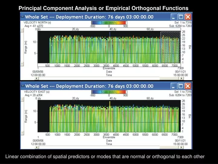
Principal Component Analysis or Empirical Orthogonal Functions. Linear combination of spatial predictors or modes that are normal or orthogonal to each other. Write data series U m (t ) = U(z, t) as :. f im are orthogonal spatial functions, also known as eigenvectors or EOFs.

E N D
Principal Component Analysis or Empirical Orthogonal Functions Linear combination of spatial predictors or modes that are normal or orthogonal to each other
Write data series Um(t) =U(z, t) as: fimare orthogonal spatial functions, also known as eigenvectors orEOFs mare each of the time series (function of depth or horizontal distance) ai(t) are the amplitudesorweightsof the spatial functions as they change in time are the eigenvalues of the problem (represent the variance explained by each mode i)
87% of variability Eigenvectors (spatial functions) or EOFs f3m f2m f1m a1 12% of variability a2
Measured Mode 1 Mode 1+2
Goal: Write data series U at any location m as the sum of M orthogonal spatial functions fim: ai is the amplitude of ith orthogonal mode at any time t For fim to be orthogonal, we require that: 2 functions are orthogonal when sum (or integral) of their product over a space or time is zero Orthogonality condition means that the time-averaged covariance of the amplitudes satisfies: (overbar denotes time average) variance of each orthogonal mode
If we form the co-variance matrix of the data Multiplying both sides times fik, summing over all k and using the orthogonality condition: Canonical form of eigenvalue problem eigenvectors eigenvalues eigenvaluesof mean product if means of Um(t) are removed
I is the unit matrix and are the EOFs Eigenvalue problemcorresponding to a linear system:
For a non-trivial solution ( 0): Sum of variances in data = sum of variance in eigenvalues