Download
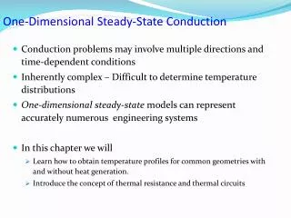
1 / 78
790 likes | 928 Views
CHAPTER 2 ONE-DIMENSIONAL STEADY STATE CONDUCTION. 2.1 Examples of One-dimensional Conduction:. 2.1.1 Plate with Energy Generation and Variable Conductivity. Example 2.1: Plate with internal energy generation. and a variabl e k. ¢. ¢. ¢. q. o. 0. C. o. 0. C. x. 0.

E N D
CHAPTER 2ONE-DIMENSIONAL STEADY STATE CONDUCTION 2.1 Examples of One-dimensional Conduction: 2.1.1 Plate with Energy Generation and Variable Conductivity
Example 2.1:Plate with internal energy generation and a variable k ¢ ¢ ¢ q o 0 C o 0 C x 0 L Fig. 2.1 Find temperature distribution. (1) Observations • Variable k • Symmetry • Energy generation • Rectangular system • Specified temperature at boundaries
(2) Origin and Coordinates Use a rectangular coordinate system (3) Formulation (i) Assumptions • One-dimensional • Steady • Isotropic • Stationary • Uniform energy generation
(2.1) (a) (b) (ii) Governing Equation Eq. (1.7): (a) into eq. (2.1) (iii) Boundary Conditions. Two BC are needed:
(c) (d) (e) (f) , (4) Solution Integrate (b) twice BC (c) and (d)
(g) (h) (i) (f) into (e) Solving for T Take the negative sign
• Limiting check: (j) (5) Checking • Dimensional check • Boundary conditions check • Symmetry Check: Setting x = L/2 in (j) gives dT/dx = 0
(k) (l) (m) • Quantitative Check Conservation of energy and symmetry: Fourier’s law at x = 0 and x = L
(n) k = constant:Set (6) Comments Solution to the special case: 2.1.2 Radial Conduction in a Composite Cylinder with Interface Friction
Example 2.2:Rotating shaft in sleeve, frictional heat at interface, convection on outside. Conduction in radial direction. Determine the temperature distribution in shaft and sleeve. (1) Observations • Composite cylindrical wall • Cylindrical coordinates • Radial conduction only
• Steady state: Energy generated = heat conducted through the sleeve • No heat is conducted through the shaft • Specified flux at inner radius of sleeve, convection at outer radius (2) Origin and Coordinates Shown in Fig. 2.2
(3) Formulation (i) Assumptions • One-dimensional radial conduction • Steady • Isotropic • Constant conductivities • No energy generation • Perfect interface contact • Uniform frictional energy flux • Stationary
(2.2) Specified flux at (a) (ii) Governing Equation Shaft temperature is uniform. For sleeve: Eq. (1.11) (iii) Boundary Conditions
(c) (d) Convection at (b) (4) Solution Integrate eq. (2.2) twice BC give C1 and C2
= Biot number (g) (e) (f) and (d) and (e) into (c) Shaft temperature T2: Use interface boundary condition
(h) • Limiting check: Evaluate (f) at r = Rsand use (g) (5) Checking • Dimensional check • Boundary conditions check (6) Comments • Conductivity of shaft does not play a role
Example 2.1:Plate 1 generates heat at Plate 1 is sandwiched between two plates. Outer surfaces of two plates at • Problem can also be treated formally as a composite cylinder. Need 2 equations and 4 BC. 2.1.1 Composite Wall with Energy Generation Find the temperature distribution in the three plates.
(1) Observations • Composite wall • Use rectangular coordinates • Symmetry: Insulated center plane • Heat flows normal to plates • Symmetry and steady state: Energy generated = Energy conducted out (2) Origin and Coordinates Shown in Fig. 2.3
(3) Formulation (i) Assumptions • Steady • One-dimensional • Isotropic • Constant conductivities • Perfect interface contact • Stationary (ii) Governing Equations Two equations:
(a) (b) (c) (d) (iii) Boundary Conditions Four BC: Symmetry: Interface:
(g) (h) (e) (f) Outer surface: (4) Solution Integrate (a) twice Integrate (b)
• Dimensional check: units of (i) (j) Four BC give 4 constants: Solutions (g) and (h) become (5) Checking
1/2 the energy generated in center plate = Heat conducted at (k) • Boundary conditions check • Quantitative check:
(l) (i) If then (ii) If then (i) into (k) Similarly, 1/2 the energy generated in center plate = Heat conducted out (j) into (l) shows that this condition is satisfied. • Limiting check:
Alternate approach: Outer plate with a specified flux at and a specified temperature at (2.3) (6) Comments 2.2 Extended Surfaces - Fins 2.2.1 The Function of Fins Newton's law of cooling:
Options for increasing • Lower • Increase • Increase h Examples of Extended Surfaces (Fins): • Thin rods on condenser in back of refrigerator • Honeycomb surface of a car radiator • Corrugated surface of a motorcycle engine • Disks or plates used in baseboard radiators
(a) constant area variable area (b) straight fin straight fin Fig. 2.5 (c) pin fin (d) annular fin 2.2.2 Types of Fins
Terminology and types • Fin base • Fin tip • Straight fin • Variable cross-sectional area fin • Spine or pin fin • Annular or cylindrical fin 2.2.3 Heat Transfer and Temperature Distribution in Fins • Heat flows axially and laterally (two-dimensional) •Temperature distribution is two-dimensional
r T ¥ d x T h , T ¥ Fig . 2 . 6 Bi = h /k << 1 (2.4) 2.2.4 The Fin Approximation Neglect lateral temperature variation Criterion: Biot number = Bi
•Assume 2.2.5 The Fin Heat Equation: Convection at Surface (1) Objective: Determine fin heat transfer rate. Need temperature distribution. (2) Procedure: Formulate the fin heat equation. Apply conservation of energy. • Select an origin and coordinate axis x. •Stationary material, steady state
(a) (b) (c) Conservation of energy for the element dx:
(d) (e) (f) (b) and (c) into (a) Fourier's law and Newton’s law Energy generation
(2.5a) (2.5b) (g) (e), (f) and (g) into (d) Assume constant k • (2.5b) is the heat equation for fins • Assumptions: (1) Steady state (2) Stationary
• and are determined from thegeometry of fin. (a) = circumference (3) Isotropic (4) Constant k (5) No radiation (6) Bi << 1 2.2.6 Determination of dAs /dx From Fig. 2.7b ds= slanted length of the element
(b) (2.6a) << 1 For (2.6b) For a right triangle (b) into (a) 2.2.7 Boundary Conditions Need two BC
2.2.8 Determination of Fin Heat Transfer Rate Conservation of energy for Two methods to determine (a)
(2.8) (2.7) (1) Conduction at base. Fourier's law at x = 0 (2) Convection at the fin surface. Newton's law applied at the fin surface • Fin attached at both ends: Modify eq. (2.7) accordingly • Fin with convection at the tip: Integral in eq. (2.8) includes tip
• Convection and radiation at surface: Apply eq. (2.7). Modify eq. (2.8) to include heat exchange by radiation. 2.2.9 Applications: Constant Area Fins with Surface Convection
(a) = constant (b) (2.9) A. Governing Equation Use eq. (2.5b). Set Eq. (2.6a) (a) and (b) into eq. (2.5b)
(c) (d) • Assume = constant, (c) and (d) into (2.9) (2.10) (2) constant k, and Rewrite eq. (2.9) Valid for: (1) Steady state
(2.11a) (2.11b) (3) No energy generation (4) No radiation (5) Bi1 (6) Stationary fin B. Solution Assume: h = constant
(e) (f) (h) C. Special Case (i): • Finite length • Specified temperature at base, convection at tip Boundary conditions:
(i) (2.12) Eq. (2.7) gives (2.13) Two BC give B1 and B2
(j) Set eq. (2.12) (2.14) Set eq. (2.13) (2.15) C. Special Case (ii): • Finite length • Specified temperature at base, insulated tip BC at tip:
• Simplified model: Assume insulated tip, compensate by increasing length by • The corrected length is (2.16) Increase in surface area due to = tip area 2.2.10 Corrected Length Lc • Insulated tip: simpler solution • The correction incrementLcdepends on the geometry of the fin: Circular fin:
2.2.11 Fin Efficiency (2.17) = total surface area Square bar of side t Definition
(2.18) Eq. (2.17) becomes 2.1.12 Moving Fins Examples: • Extrusion of plastics • Drawing of wires and sheets • Flow of liquids
(a) (b) Heat equation: Assume: • Steady state • Constant area • Constant velocity U • Surface convection and radiation Conservation of energy for element dx
(c) (d) (e) (f) (g) (2.19) Fourier’s and Newton’s laws (b)-(g) into (a) assume constant k
(2) Constant U, k, Pand Assumptions leading to eq. (2.19): (1) Steady state (3) Isotropic (4) Gray body (5) Small surface enclosed by a much larger surface and (6) Bi << 1