Download

1 / 42
420 likes | 565 Views
Selecting Input Distribution. Introduction. The data on the input random variables of interest can be used in following ways: The data values themselves are used directly in the simulation. This is called trace-driven simulation.

E N D
Introduction The data on the input random variables of interest can be used in following ways: • The data values themselves are used directly in the simulation. This is called trace-driven simulation. • The data values could be used to define an empirical distribution function in some way. • Standard techniques of statistical inferences are used to “fit” a theoretical distribution form to the data and perform hypothesis tests to determine the goodness of fit.
Different approaches • Approach 1 is used to validate simulation model when comparing model output for an existing system with the corresponding output for the system itself. • Two drawbacks of approach 1: simulation can only reproduce only what happened historically; and there is seldom enough data to make all simulation runs. • Approach 2 avoids these shortcomings so that any value between minimum and maximum can be generated. So approach 2 is preferred over approach 1. • If theoretical distributions can be found that fits the observed data (approach 3), then it is preferred over approach 2.
Different approaches Approach 3 vs. approach 2: • Empirical distribution may have some irregularities if small number of data points are available. Approach 3 smoothens out the data and may provide information on the overall underlying distribution. • In approach 2, it is usually not possible to generate values outside the range of observed data in the simulation. • If one wants to test the performance of the simulated system under extreme conditions, that can not be done using approach 2. • There may be compelling (physical) reasons in some situations for using a particular theoretical distribution. In that case too, it is better to get empirical support for that distribution from the observed data.
Different approaches Approach 3 vs. approach 2: • Theoretical distribution is a compact way of representing a set of data values. • In approach 2, if n data points are available from a continuous distribution, then 2n values (data and the corresponding cumulative distribution function values) must be entered and stored in the computer to represent the empirical distribution in many simulation languages. Imagine the trouble, if a large data set of observed values is present!
Sources of randomness for common simulation experiments • Manufacturing: processing times, machine operating times before a downtime, machine repair times etc. • Computer: inter-arrival times of jobs, job types, processing requirements of jobs etc. • Communication: inter-arrival times of messages, message types and lengths etc. • Mechanical systems: fluid flow in pipes, accumulation of dirt on the pipe walls, manufacturing defect size and location on a mechanical boundary, etc.
Parameters of distribution • A location parameter specifies an abscissa location point of a distributions range of values. Usually, it is the midpoint (e.g. mean) or lower endpoint of the distribution’s range. • As location parameter changes the associated distribution merely shifts left or right without otherwise changing. • A scale parameter determines the scale (or unit) of measurement of the values in the range of distribution. • A change in scale parameter compresses or expands the associated distribution without altering its basic form.
Parameters of distribution • A shape parameter determines, distinct from location and scale, the basic form or shape of a distribution within the general family of distributions. • A change in shape parameter alters a distribution’s characteristics (e.g. skewness) more fundamentally than a change in location or scale. • Some distributions (e.g. normal, exponential) do not have a shape parameter, while others have several (beta distribution has two).
Empirical distributions For ungrouped data: • Let X(i) denote the ith smallest of the Xj’s so that:
Empirical distributions For grouped data: • Suppose that nXj’s are grouped in k adjacent intervals [a0,a1), [a1,a2),…[ak-1,ak) so that jth interval contains nj observations. n1+ n2+… nk = n. • Let a piecewise linear function G be such that G(a0) = 0, G(aj) = (n1+ n2+… nj) /n, then:
Verifying Independence • Most of the statistical tests assume IID input. • At times, simulation experiments have input that are, by default dependent: e.g. hourly temperature in a city. • Two graphical ways of studying independence: • Correlation plot: Plot of ρj for j = 0, 1,2, … l. If ρj the differ from 0 by a significant amount, then this is strong evidence that the Xi’s are not independent. • Scatter plot: Plot of the pair (Xi, Xi+1) for i = 1,2,…n-1. If Xi’s are independent, then this plot would have points scattered randomly. Trend would indicate dependency.
Clues from summary statistics • For the symmetric distributions mean and median should match. In the sample data, if these values are sufficiently close to each other, we can think of a symmetric distribution (e.g. normal). • Coefficient of variation (cv): (ratio of std dev and the mean) for continuous distributions. The cv = 1 for exponential dist. If the histogram looks like a slightly right-skewed curve with cv >1, then lognormal could be better approximation of the distribution. Note: For many distributions cv may not even be properly defined. When? Examples?
Clues from summary statistics • Lexis ratio: same as cv for discrete distributions. • Skewness (ν): measure of symmetry of a distribution. For normal dist. ν = 0. For ν>0, the distribution is skewed towards right (exponential dist, ν = 2). And for ν<0, the distribution is skewed towards left.
Practical example • Data points: 217. • For these data points, we need to fit a probability distribution so that simulation experiment can be performed.
Parameter estimation • We assume that the observations are IID. • Let θ be the parameter (unknown) of the hypothesized distribution. • With this parameter, the probability of observing the data we observe is called the likelihood function. • Our task is find the parameters such that it maximizes this likelihood function, since we have already observed the data. These parameters are called Maximum Likelihood Estimators (MLE).
Parameter estimation: Exponential dist. • Hence, for exponential distribution, the MLE parameter is just the sample mean.
Parameter estimation • We can clearly see that for a distribution with more than one parameters, the MLE calculations become significantly difficult. • Normal distribution is a notable exception to the above, though.
Goodness-of-fit • For the input data we have, we have assumed a probability distribution. • We also have estimated the parameters for the same. • How do we know this fitted distribution is “good enough?” • It can be checked by several methods: • Frequency comparison • Probability plots • Goodness-of-fit tests
Frequency comparison • Graphical comparison of a histogram of the data with the density function f(x) of the fitted distribution. • Let [b0,b1), [b1,b2), …[bk-1, bk) be a set of k histogram intervals each with width = bj – bj-1. • Let hj be the observed proportion of Xi’s in the jth interval. • Let rj be the expected proportion of the n observations that would fall in the jth interval if the fitted distribution were the true one.
Frequency comparison • Then the frequency comparison is made by plotting both hj and rj in the jth histogram interval for j = 1, 2, …k. • For discrete distribution, the concept is same; except here: rj= p(xj).
Probability plots • Q-Q plot: Quantile-quantile plot • Graph of the qi-quantile of a fitted (model) distribution versus the qi-quantile of the sample distribution. • If F^(x) is the correct distribution that is fitted, for a large sample size, then F^(x) and Fn(x) will be close together and the Q-Q plot will be approximately linear with intercept 0 and slope 1. • For small sample, even if F^(x) is the correct distribution, there will some departure from the straight line.
Probability plots • P-P plot: Probability-Probability plot. • It is valid for both continuous as well as discrete data sets. • If F^(x) is the correct distribution that is fitted, for a large sample size, then F^(x) and Fn(x) will be close together and the P-P plot will be approximately linear with intercept 0 and slope 1.
Probability plots • The Q-Q plot will amplify the differences between the tails of the model distribution and the sample distribution. • Whereas, theP-P plot will amplify the differences at the middle portion of the model and sample distribution.
Goodness-of-fit tests • A goodness-of-fit test is a statistical hypothesis test that is used to assess formally whether the observations X1, X2, X3…Xn are an independent sample from a particular distribution with function F^. H0: The Xi’s are IID random variables with distribution function F^. • Two famous tests: • Chi-square test • Kolmogorov - Smirnov test
Chi-square test • Applicable for both: continuous as well as discrete distributions. • Method of calculating chi-square test statistic: • Divide the entire range of fitted distribution into k adjacent intervals -- [a0 ,a1), [a1,a2),…[ak-1,ak), where it could that a0 = -∞ in which case the first interval is (-∞,a1) and/or ak = ∞. Nj = # of Xi’s in the jth interval [aj-1,aj), j= 1,2…n. • Next, we compute the expected proportion of Xi’s that would fall in the jth interval if we were sampling from fitted distribution
Chi-square test • Finally the test statistic is calculated as:
Chi-square test • This calculated value of the test statistic is compared with the tabulated value of chi-square distribution with k-1 df at 1-α level of significance.