Download
1 / 26
260 likes | 382 Views
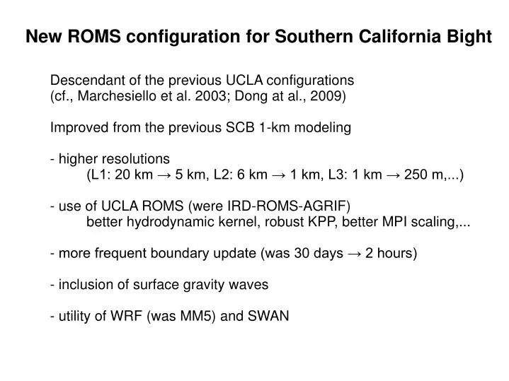
New ROMS configuration for Southern California Bight. Descendant of the previous UCLA configurations (cf., Marchesiello et al. 2003; Dong at al., 2009) Improved from the previous SCB 1-km modeling - higher resolutions (L1: 20 km → 5 km, L2: 6 km → 1 km, L3: 1 km → 250 m,...)

E N D
New ROMS configuration for Southern California Bight Descendant of the previous UCLA configurations (cf., Marchesiello et al. 2003; Dong at al., 2009) Improved from the previous SCB 1-km modeling - higher resolutions (L1: 20 km → 5 km, L2: 6 km → 1 km, L3: 1 km → 250 m,...) - use of UCLA ROMS (were IRD-ROMS-AGRIF) better hydrodynamic kernel, robust KPP, better MPI scaling,... - more frequent boundary update (was 30 days → 2 hours) - inclusion of surface gravity waves - utility of WRF (was MM5) and SWAN
Newest quadruple Nested ROMS configuration L1 (5 km) L3 (250 m) L2 (1 km) L2 (1 km) L4 (75 m) L3 (250 m) L4 (75 m)
L3 (250 m) runs (Aug. - Nov., 2006)
Effects of surface waves (subtidal EKE) w/o wave w/ wave difference
Conservative Wave Effects: Overall Thermocline Deepening and Altering Upper Mean Circulation with WEC (with WEC) –(no WEC) (m) mean mixed-layer depth (KPP hbl) ~15 % with WEC (with WEC) –(no WEC) mean stream function (upper layer > -25 m) ~15 % x 103 (m2/s)
Vortex force vs. Stokes-Coriolis effect Ro= ~ <JVF>/<JSC> - mean advection of eddies (JSC : Stokes-Coriolis force) - eddy-wave interaction (JVF : vortex force) --> exceeds JSC
L4 (75 m) runs (Aug. - Nov., 2006) HTP 1-/5-mile outfalls
Mean mixed layer depth (from KPP)
Hovmoller plots of depth-averaged tracer concentration
Alongshore profiles of depth-averaged tracer concentration at the shoreline
Time series of depth-averaged tracer concentration at the shoreline at selected locations.
Single-point PDF of depth-averaged passive tracer concentrations at the shore
PSD of depth-averaged passive tracer concentrations at the shoreline
Hovmoller plots of shoreline SSS
Mean surface normalized relative vorticity and TKE (all frequencies)
bandpass-filtered surface kinetic energy high frq. (< 8h) semi-diurnal diurnal sub-tidal (> 36h)
L5 (20 m) test run (7 days in Nov., 2006)