Download
1 / 48
480 likes | 570 Views
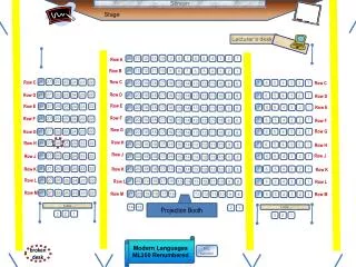
Stage. Screen. Lecturer’s desk. 11. 10. 9. 8. 7. 6. 5. 2. 14. 13. 12. 4. 3. 1. Row A. 14. 13. 12. 11. 10. 9. 6. 8. 7. 5. 4. 3. 2. 1. Row B. 28. 27. 26. 23. 25. 24. 22. Row C. 7. 6. 5. Row C. 2. 4. 3. 1. 21. 20. 19. 18. 17. 16. 13. Row C. 15.

E N D
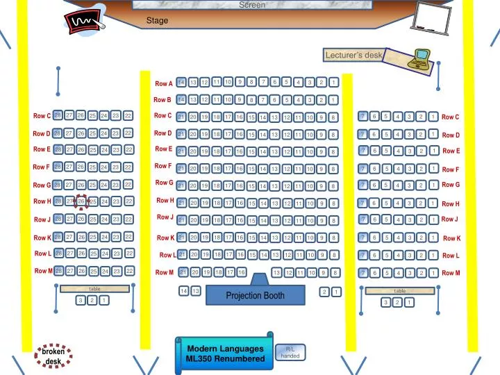
Stage Screen Lecturer’s desk 11 10 9 8 7 6 5 2 14 13 12 4 3 1 Row A 14 13 12 11 10 9 6 8 7 5 4 3 2 1 Row B 28 27 26 23 25 24 22 Row C 7 6 5 Row C 2 4 3 1 21 20 19 18 17 16 13 Row C 15 14 12 11 10 9 8 22 27 28 26 25 24 23 Row D 1 Row D 6 21 20 19 18 17 16 13 7 5 4 3 2 15 14 12 11 10 9 8 Row D Row E 28 27 26 22 Row E 23 25 24 7 6 5 1 2 4 3 Row E 21 20 19 18 17 16 13 15 14 12 11 10 9 8 Row F 28 27 26 23 25 24 22 Row F 1 6 21 20 19 18 17 16 13 7 5 4 3 2 15 14 12 11 10 9 8 Row F Row G 22 27 28 26 25 24 23 7 6 5 1 Row G 2 4 3 Row G 21 20 19 18 17 16 13 15 14 12 11 10 9 8 Row H 28 27 26 22 23 25 24 Row H 6 21 20 19 18 17 16 13 7 5 4 3 2 1 15 14 12 11 10 9 8 Row H Row J 28 27 26 23 25 24 22 7 6 5 Row J 2 4 3 1 Row J 21 20 19 18 17 16 13 15 14 12 11 10 9 8 22 27 28 26 25 24 23 6 21 20 19 18 17 16 13 7 5 4 3 2 1 15 14 12 11 10 9 8 Row K Row K Row K 28 27 26 22 23 Row L 25 24 21 20 19 18 17 16 13 6 15 14 12 11 10 9 8 Row L 7 5 4 3 2 1 Row L 28 27 26 22 23 Row M 25 24 21 20 19 18 17 16 13 6 12 11 10 9 8 Row M 7 5 4 3 2 1 Row M table • Projection Booth 14 13 2 1 table 3 2 1 3 2 1 Modern Languages ML350 Renumbered R/L handed broken desk
Use this as your study guide By the end of lecture today1/26/12 Surveys and questionnaire design Simple versus systematic random sampling Sample frame and randomization Stratified sampling Cluster sampling Judgment sampling Snowball sampling, convenience sampling Time series design vs. Cross sectional design Correlations
Schedule of readings Before next exam: Please read chapters 1 - 4 & Appendix D & E in Lind Please read Chapters 1, 5, 6 and 13 in Plous Chapter 1: Selective Perception Chapter 5: Plasticity Chapter 6: Effects of Question Wording and Framing Chapter 13: Anchoring and Adjustment
MGMT 276: Statistical Inference in ManagementRoom 350 Modern LanguagesSpring, 2012 Welcome http://www.youtube.com/watch?v=Ahg6qcgoay4&watch_response
Two Homework assignments due at same time – Tuesday (January 31st) On class website: please print the worksheetthat describes homework assignments 2 & 3 Please double check – Allcell phones other electronic devices are turned off and stowed away
Review of 5 Principles of questionnaire construction 1. Identify what constructs 2. Consider their sensibilities of your responders 3. Assessment should feel easy and clear, unthreatening 4. Avoid ambiguity and bias in your items 5. Consider lots of different formats for responses
5 Principles of questionnaire construction 5. Consider lots of different formats for responses • Consider open-ended vsclosed-ended questions - pros and cons of each - can often modify a question into a closed question • Consider complementing your questionnaire with other forms of data collection (focus group or direct observation) • Pilot – feedback – fix - pilot – analyze – fix - pilot – etc Respect process of empirical approach
Likert Rating scales: measure that allows for rating the level of agreement with a statement. The score reflects the sum of responses on a series of items. Rating scales: a continuum of response choices Anchored rating scales: a written description somewhere on the scale I prefer rap music to classical music Agree 1---2---3---4---5 Disagree Fully anchored rating scales: a written description for each point on the scale I prefer rap music to classical music 1---------2---------3---------4---------5 StronglyDisagree StronglyAgree Agree Disagree Neutral
Summated scales - miniquiz (like Cosmo - ask several questions then sum responses) - For example, several questions on political views (coded so that larger numbers mean “more liberal”) 1. The rights of the community are more important than rights of any one individual agree 1 --- 2 --- 3 --- 4 --- 5 disagree 2. Marriage should be between one man and one woman agree 1 --- 2 --- 3 --- 4 --- 5 disagree 3. Evolution has no place in public education agree 1 --- 2 --- 3 --- 4 --- 5 disagree
Ranking scales Rank options in ascending or descending order An apartment / house should have ___ lots of square feet ___ access to bus route ___ pleasant neighbors ___ workshop / workout area ___ big rooms ___ close to work / school Note: Options can come from open-ended questions or surveys
Semantic differential Create a profile of your opinion An apartment / house should be (place checkmarks) Cozy and small___ _______________roomy and large Quiet ___ _______________Active community Larger communal rooms ___ _______________Larger bedrooms Note: Options can come from open-ended questions or surveys
Checklist An apartment / house should have ___ lots of square feet ___ access to bus route ___ pleasant neighbors ___ workshop / workout area ___ big rooms ___ close to work / school Note: Options can come from open-ended questions or surveys
Questionnaires use self-report items for measuring constructs. Constructs are operationally defined by content of items. Questionnaire is a set of fixed-format, self-report items completed without supervision or time-constraint Response rate and power of random sampling Number of responders versus percentage of responders Really important regarding bias! Wording, order, balance can all affect results
Questionnaires use self-report items for measuring constructs. Constructs are operationally defined by content of items. As “consumers” of questionnaire data – what should we ask? Number of responders versus percentage of responders Methodology of sampling Operational definitions of constructs Wording As “composers” of questionnaire data – how should we ask? - pilot – fix - pilot – analyze – fix - pilot – all the way through your design
Interviews Interview often a survey is read to a participant either over the phone or in person Which is better: on phone or in person? Pros: Cons: Unstructured interview Structured interview Which is better: structured or unstructured? Pros: Cons: Focus group
Questionnaire Homework
Questionnaire Homework
Questionnaire Homework
Questionnaire Homework Variable label and scale values Variable label and scale values
Questionnaire Homework What might you graph?
Sample versus census How is a census different from a sample? Census measures each person in the specific population Sample measures a subset of the population and infers about the population – representative sample is good What’s better? Use of existing survey data U.S. Census Family size, fertility, occupation The General Social Survey Surveys sample of US citizens over 1,000 items Same questions asked each year
Population (census) versus sampleParameter versus statistic Parameter – Measurement or characteristic of the population Usually unknown (only estimated) Usually represented by Greek letters (µ) pronounced “mu” pronounced “mew” Statistic – Numerical value calculated from a sample Usually represented by Roman letters (x) pronounced “x bar”
“Random Sampling Technique” Simple random sampling: each person from the population has an equal probability of being included Sample frame = how you define population Let’s take a sample …a random sample Question: Average weight of U of A football player Sample frame population of the U of A football team Pick 24th name on the list Random number table – List of random numbers Or, you can use excel to provide number for random sample =RANDBETWEEN(1,110) Pick 64th name on the list(64 is just an example here) 64
“Random Sampling Technique” Systematic random sampling: A probability sampling technique that involves selecting every kth person from a sampling frame You pick the number Other examples of systematicrandom sampling 1) check every 2000th light bulb 2) survey every 10th voter
“Random Sampling Technique” Stratified sampling: sampling technique that involves dividing a sample into subgroups (or strata) and then selecting samples from each of these groups - sampling technique can maintain ratios for the different groups Average number of speeding tickets 12% of sample is from California 7% of sample is from Texas 6% of sample is from Florida 6% from New York 4% from Illinois 4% from Ohio 4% from Pennsylvania 3% from Michigan etc Average cost for text books for a semester 17.7% of sample are Pre-business majors 4.6% of sample are Psychology majors 2.8% of sample are Biology majors 2.4% of sample are Architecture majors etc
“Random Sampling Technique” Cluster sampling: sampling technique divides a population sample into subgroups (or clusters) by region or physical space. Randomly select samples for each cluster Textbook prices Southwest schools Midwest schools Northwest schools etc Average student income, survey by Old main area Near McClelland Around Main Gate etc Patient satisfaction for hospital 7th floor (near maternity ward) 5th floor (near physical rehab) 2nd floor (near trauma center) etc
These are not “Random Sampling Techniques” Convenience sampling: sampling technique that involves sampling people nearby. A non-random sample and vulnerable to bias Snowball sampling: a non-random technique in which one or more members of a population are located and used to lead the researcher to other members of the population Used when we don’t have any other way of finding them Also vulnerable to biases
These are not “Random Sampling Techniques” Judgment sampling: sampling technique that involves sampling people who an expert says would be useful. A non-random sample and vulnerable to bias
Designed our study / observation / questionnaire Collected our data Organize and present our results
Scatterplot displays relationships between two continuous variables Correlation: Measure of how two variables co-occur and also can be used for prediction Range between -1 and +1 The closer to zero the weaker the relationship and the worse the prediction Positive or negative
Correlation Range between -1 and +1 +1.00 perfect relationship = perfect predictor +0.80 strong relationship = good predictor +0.20 weak relationship = poor predictor 0 no relationship = very poor predictor -0.20 weak relationship = poor predictor -0.80 strong relationship = good predictor -1.00 perfect relationship = perfect predictor
Positive correlation: as values on one variable go up, so do values for the other variable Negative correlation: as values on one variable go up, the values for the other variable go down Height of Mothers by Height of Daughters Height ofMothers Positive Correlation Height of Daughters
Positive correlation: as values on one variable go up, so do values for the other variable Negative correlation: as values on one variable go up, the values for the other variable go down Brushing teeth by number cavities BrushingTeeth Negative Correlation NumberCavities
Perfect correlation = +1.00 or -1.00 One variable perfectly predicts the other Height in inches and height in feet Speed (mph) and time to finish race Positive correlation Negative correlation
Correlation The more closely the dots approximate a straight line,(the less spread out they are) the stronger the relationship is. Perfect correlation = +1.00 or -1.00 One variable perfectly predicts the other No variability in the scatterplot The dots approximate a straight line
Correlation does not imply causation Is it possible that they are causally related? Yes, but the correlational analysis does not answer that question What if it’s a perfect correlation – isn’t that causal? No, it feels more compelling, but is neutral about causality Number of Birthdays Number of Birthday Cakes
Positive correlation: as values on one variable go up, so do values for other variable Negative correlation: as values on one variable go up, the values for other variable go down Number of bathrooms in a city and number of crimes committed Positive correlation Positive correlation
Linear vs curvilinear relationship Linear relationship is a relationship that can be described best with a straight line Curvilinear relationship is a relationship that can be described best with a curved line
Correlation - How do numerical values change? http://neyman.stat.uiuc.edu/~stat100/cuwu/Games.html http://argyll.epsb.ca/jreed/math9/strand4/scatterPlot.htm Let’s estimate the correlation coefficient for each of the following r = +.80 r = +1.0 r = -1.0 r = -.50 r = 0.0
This shows the strong positive (.8) relationship between the heights of daughters (measured in inches) with heights of their mothers (measured in inches). 48 52 5660 64 68 72 Both axes and values are labeled Both axes and values are labeled Both variables are listed, as are direction and strength Height of Mothers (in) 48 52 56 60 64 68 72 76 Height of Daughters (inches)
Break into groups of 2 or 3 Each person hand in own worksheet. Be sure to list your name and names of all others in your group Use examples that are different from those is lecture 1. Describe one positive correlation Draw a scatterplot (label axes) 2. Describe one negative correlation Draw a scatterplot (label axes) 3. Describe one zero correlation Draw a scatterplot (label axes) 4. Describe one perfect correlation (positive or negative) Draw a scatterplot (label axes) 5. Describe curvilinear relationship Draw a scatterplot (label axes)
Both variables are listed, as are direction and strength Both axes and values are labeled Both axes and values are labeled This shows the strong positive (.8) relationship between the heights of daughters (measured in inches) with heights of their mothers (measured in inches). 48 52 5660 64 68 72 1. Describe one positive correlation Draw a scatterplot (label axes) Height of Mothers (in) 2. Describe one negative correlation Draw a scatterplot (label axes) 48 52 56 60 64 68 72 76 Height of Daughters (inches) 3. Describe one zero correlation Draw a scatterplot (label axes) 4. Describe one perfect correlation (positive or negative) Draw a scatterplot (label axes) 5. Describe curvilinear relationship Draw a scatterplot (label axes)
Thank you! See you next time!!