Download
1 / 105
1.2k likes | 1.64k Views
Network calculus :. Jean-Yves Le Boudec and Patrick Thiran LCA-ISC, I&C, EPFL. CH-1015 Lausanne Jean-Yves.Leboudec Patrick.Thiran @epfl.ch http://lcawww.epfl.ch. Contents. 1. Greedy shapers and arrival curves, min-plus convolution 2. Service curves, backlog, delay bounds

E N D
Network calculus : Jean-Yves Le Boudec and Patrick Thiran LCA-ISC, I&C, EPFL CH-1015 Lausanne Jean-Yves.Leboudec Patrick.Thiran @epfl.ch http://lcawww.epfl.ch
Contents 1. Greedy shapers and arrival curves, min-plus convolution 2. Service curves, backlog, delay bounds 3. Diffserv: intuition and formal definition behind EF 4. Min-plus algebra in action: Video smoothing 5. Statistical multiplexing with EF free on-line at : http://lcawww.epfl.ch
What is Network Calculus ? • Deterministic analysis of queuing / flow systems arising in communication networks • Uses Min-Plus, Max-Plus and sometimes Min-Max algebra
The standard Linear Theory • A LTI filter in conventional algebra (R, +, ×) • Input signal = electrical voltage x(t) • System = circuit (filter) with impulse response b(t) • Output = convolution of x(t) and b(t) :y(t) = b(t-s) x(s) ds + + x(t) b(t) y(t) - -
CBR shaper x(t) y(t) bit rate c Network Calculus uses Min-Plus Linear Theory • A linear system in min-plus algebra (R, min, +) • Input = arrived traffic in [0,t], x(t) • System = CBR trunk of rate c : b(t) = ct • Output = convolution ofx(t) and b(t):y(t) = infs {b(t-s)+ x(s) }
Two key ConceptsArrival and Service Curves • IntServ and DiffServ use the concepts of arrival curve and service curves
Contents • Arrival curves • Arrival curve: definition • Leaky bucket and GCRA • Arrival curve and min-plus convolution • Good arrival curves are sub-additive • Minimal arrival curve and min-plus deconvolution • Greedy shaper and its properties • Packetization 2. Service curves, GPS, backlog, delay bounds 3. Diffserv: intuition and formal definition behind EF 4. Min-plus algebra in action: Video smoothing 5. Statistical multiplexing with EF
Cumulative flows • Cumulative flow R(t) F , t real or integer • F = { x(t) | x(t) is non decreasing and x(t) = 0 for t < 0 } • Examples: bits bits bits R1(t) R2(t) R3(t) 1 2 5 6 7 1 5 5.5 1 2 5 6 time t time t time t Discrete-time model (left continuous) Fluid model (continuous) Packet model (left continuous)
Example • MPEG files, 25 frames/sec R R
bits slope r b time Arrival Curves • Arrival curve For any times 0 st, the cumulative flow R(.) satisfies R(t) -R(s) (t-s) Example 1: affine arrival curve gr,b (t) = gr,b(t) = rt+b for t>0 R(t)
Arrival Curves Example 2: stair arrival curvekvT,t • (t) = kvT,t (t) =k(t+t)/T with T = period, t = tolerance, k = constant packet size • Characterizes flows that are periodic stream of packets of same size k (cells), that suffers a variable delay <=t kvT,t(t) = k(t+t)/T bits • All packets of size k. Then R conforms to =kvT,t • R conforms to = gr,b with r = k/T and b = k(t+T)/T 4k 3k 2k k 3T-t t 2T-t T-t time
Leaky bucket • All packets of flow R are declared conformant by a leaky buket controller of rate r and size b R conforms to (t) = gr,b(t) = rt+b for t>0 R(t) gr,b R(t) R(t) slope r b b b x(t) x(t) t 1 5 5.5 r
GCRA (T,t) • All packets (cells) of flow R are of the same size k • Arrival time of nth = An • Theoretical arrival just after nth arrival is qn = max(An,qn-1) + T • If An+1 >= qn – t then cell is conformant, otherwise not Example: GCRA (10,2) n 1 2 3 3 4 5 qn-1 0 11 21 21 31 41 An 1 11 16 20 29 38 c c nc c c nc • Equivalences: R conforms toGCRA (T,t) R conforms to staircase arrival curve = kvT,t R conforms toleaky bucket (r = k/T, b = k(t+T)/T) • R conforms toaffine arrival curve = gr,b
bits bits slope r slope r b b slope m M time time Combining leaky buckets • standard arrival curve in the Internet ( = min)(u) = min (pu+M, ru+b) = (pu+M) (ru+b)
If ais an arrival curve for flow R, so is a • a(t) a(t) • What isa(t) ? • The answer uses min-plus convolution and sub-additivity a(t) a(t) 4k 4k 3k 3k 2k 2k k k 3T 3T 2T 2T T T 4T 4T Sub-additivity and arrival curves
(f g)(t) Min-plus convolution • Definition (fg) (t) = infu { f(t-u) + g(u) } g(t) f(t) t
f(t) R f(s) K t (fg)(t) T (fg)(t) r K+b g(t-s) K R s t T Example (fg) (t) = ? g(t) r t b t
Some properties of min-plus convolution • (f g) F • is associative • is commutative • Neutral element: 0 : f 0 = f(0 (t) = 0 for t = 0 and 0 (t) = for t > 0) • is distributive with respect to min () • is isotone: f f’ and g g’ fg f’g’ • Functions passing through the origin (f(0) = g(0) = 0): fg f g • Concave functions passing through the origin: fg = f g • Convex piecewise linear functions: fg is the convex piecewise linear function obtained by putting end-to-end all linear pieces of f and g, sorted by increasing slopes
lR(t)=Rt dT(t) bR,T(t) Slope (rate) R Rate R delay T latency T bR,T is convex (rate-latency function) lR is convex (delay function) Example: rate latency function dT is convex (delay function) =
f(t) R f = K + bR,T = K + T lR K t T g(t) g = gr,b =0 (lr +b) concave with g(0) = 0 (fg)(t) r r K+b b K R t t T Example bis (using rules) fg = (K + TlR) gr,b = K + ((TlR) gr,b) = K + (T(lR gr,b )) = K + (T(lRgr,b )) = K + (TlR ) (Tgr,b ) = K + bR,T (Tlr +b) = K + bR,T (br,T +b)
We can express arrival curves with min-plus convolution • Arrival Curve property means for all 0 st, x(t) -x(s) (t-s) x(t) x(s) +(t-s) for all 0 st x(t) infu { x(u) + (t-u) } x x
Sub-additive function • f is sub-additive f (t) + f(s) f(t+s) • f is concave with f(0) = 0 f is sub-additive • f is sub-additive f is concave • f,g are sub-additive and pass through the origin (f(0) = g(0) = 0) fg is sub-additive
Examples bits gr,b is concave vT,t (t) bits gr,b(t) 4k 3k slope r 2k b k 3T-t t 2T-t T-t time time vT,t is not concave, but is sub-additive
Sub-additive closure • f = inf {0 ,f,f f, f f f,… } • f is sub-additive with f(0) = 0 • f is sub-additive with f(0) = 0 f =f f = f f
(bR,T(t)+K’)(2) bR,T(t)+K’ 2K’ (bR,T(t)+K’)(2) bR,T(t)+K’’ Examples bits bits bR,T(t)+K’’ bR,T(t)+K’ R R K’ K’’ T 2T T 2T time time
What isa(t) ? • can be replaced by its sub-additive closure a. • From now on: we will always take sub-additive arrival curves passing through the origin. a(t) Sub-additivity and arrival curves bits a(t) 4k 3k 2k k 3T 3T 2T 2T T T 4T 4T
Minimal arrival curve • If the only available information on a flow is obtained from measurements, i.e if we only know R, how can we compute its minimal arrival curve a ? • The answer uses min-plus deconvolution R
(f g)(t) g(t) Min-plus deconvolution Ø • Definition (fØg) (t) = supu { f(t+u) - g(u) } f(t) t
Some properties of min-plus deconvolution • (fg) F in general • (ff) F • (ff) is sub-additive with (ff) (0) = 0 • (fg) h = f (g h) • Duality with : fg h f g h
Minimal arrival curve • The minimal arrival curve of flow R is a = RØR. • Proof: • It is an arrival curve because R(t) – R(s) = R((t-s)+s) - R(s) supu { R((t-s)+u) - R(u) } = (R ØR) (t-s) • If ’ is another arrival curve for flow R, then R R ’ R Ø R ’ so that ’ .
Example • MPEG files, 25 frames/sec R R
Greedy shaper Shaper R(t) x(t) s Definition of Greedy shaper • forces output to be constrained by arrival curve x(t) - x(s) s(t - s) • storesdata in a buffer if needed • Hence the shaper maximises x(t) such thatx(t)R(t)x(t)(xs(t)
Shaper R(t) x(t) s Output of a Greedy shaper • If s is sub-additive and s(0) = 0, x = Rs • Proof: • x = R s is a solution because x= R sR sinces(0) = 0 x= R s = R (s s) =(R s s = x s • If x’ is another solution then x’ R and x’ x’s . Combining the two and using isotonicity of :x’ x’s Rs = x
+ + y(t) x(t) s(t) - - y x shaper s Greedy shaper = linear min-plus filter • Standard convolution in (R, x, +) (LTI filter) y(t)=(s * x)(t) = s(t-u) x(u) du • Min-plus convolution in (R, +, ) is linear ( = min) y(t) = (sx) (t) = infu { s(t-u) + x(u) }
Shaper R(t) x(t) s What is done by shaping cannot be undone by shaping • Suppose that R(t) is constrained by arrival curve a : R R a . • Then x =R s (R a)s = R (a s) R a since s(0) = 0. • Therefore shaping keeps arrival constraints. • In fact, the output flow has a s as arrival curve a-smooth
Packetization • The shaper presented before is for constant size packets or ideal fluid systems • Real life systems are modelled by adding a packetizer transforms fluid input into packets of size l1, l2, l3, … • Packetizer adds some distortion, well understood R*(t) l1 l2 l1 l3 l2 l3 R(t) (PL ) c l1 + l2 + l3 R’(t) l1 + l2 constant rate server = greedy shaper s(t)=ct + packetizer l1 T1 T2 T3
Contents • Arrival curves 2. Service curves, backlog, delay bounds • Service curve: definition • Backlog and delay bounds • Guaranteed Rate Servers • Application to IntServ • Application to Core-Stateless 3. Diffserv: intuition and formal definition behind EF 4. Min-plus algebra in action: Video smoothing 5. Statistical multiplexing with EF
Goal of Service Curve and GR node definitions • define an abstract node model • independent of a specific type of scheduler • applies to real routers, which are not a single scheduler, but a complex interconnection of delay and scheduling elements • applies to nodes that are not work-conserving
S x y b(t) y x y(t) x(s) t s Service Curve • System S offers a (minimal) service curve to a flow iff for all t there exists some s such that y(t) - x(s) (t-s)
The constant rate server has service curve b(t)=ct Proof: take s = beginning of busy period: y(t) – y(s) = c (t-s) and y(s) = x(s) -> y(t) – x(s) = c (t-s) ct buffer t s t 0
Shaper x(t) y(t) s The service curve of a Greedy shaper is its shaping curve • If s is sub-additive and s(0) = 0, y(t) = (xs(t). • The service curve of a shaper is thuss.
x y T seconds The guaranteed-delay node has service curve dT T (t) t 0 T Function T
The standard model for an Internet router • rate-latency service curve bits R T seconds
We can express service curves with min-plus convolution • Service Curve guarantee means there exists some 0 st : y(t) - x(s) (t-s) y(t) x(s) +b(t-s) for some 0 st y(t) infu { x(u) + b(t-u) } y x
Tight Bounds on delay and backlog If flow has arrival curve and node offers service curve then • backlog sup ((s) -(s)) = (Ø)(0) =v(, ) • delay inf { s 0 : (Ø)(-s) 0 } = h(, ) h(,) v(,)
The composition theorem • Theorem: the concatenation of two network elements each offering service curve i offers the service curve 12
R1 = R1 R2 T1 T2 T2 T1+T2 Example • tandem of routers
D1 D2 D Pay Bursts Only Once D1+D2 (2b + RT1)/ R + T1 + T2 Db /R + T1 + T2 end to end delay bound is less
end-to-end service curve 2 2 a Shaper 2 s2 a s a Re-shaping is for free • Re-shaper is added to re-enforce some fraction of the original constraint • Delay for original system = h(, 2) • For system with re-shaper = h(, s2) = h(, s2) • Now h(, s2) = h(, 2) interpretation: put re-shaper before node 1; it is transparent formal proof uses delay =inf { d : Ø( 2) (-d) 0 } • Therefore delay bound for both systems are equal
Guaranteed Rate node • An alternative definition to service curve for FIFO • for rate-latency service curves only • Definition (Goyal, Lam, Vin; Chang): a node is GR(r,e) if D(n) F(n) + e F(n) = max{A(n), F(n-1)} + L(n)/r D(n) : departure time for packet nA(n) : arrival timeF(n) : virtual finish time, F(0) = 0L(n) : length in bits for packet n