Download

1 / 23
230 likes | 346 Views
Abstract Reasoning of Programs Part 2. Francis Tang March 21, 2003. References. [CLRS] Cormen, Leiserson, Rivest and Stein, Introduction to Algorithms 2 nd Ed , MIT Press, 2001.

E N D
Abstract Reasoning of ProgramsPart 2 Francis Tang March 21, 2003
References [CLRS] Cormen, Leiserson, Rivest and Stein, Introduction to Algorithms 2nd Ed, MIT Press, 2001. [Gusfield] Gudfield, Algorithms on Strings, Trees , and Sequences: Computer Science and Computational Biology, CUP, 1997. (The BII Library has a copy of this book.)
Revision: Motivation • Want to apply rigour to programming • Need a feasible technique for reasoning about complex algorithms • We need abstraction to be able to feasibly reason about complex algorithms • Should be language independent
Objectives • Demonstrate loop invariant arguments by example • Provide you with the foundations to be able to reason about while-loop algorithms/programs • Provide you with enough background to be able to understand other people’s reasoning • Show you how abstraction can give simplifications
Non-objectives (sorry) • Teach you about programming in Java/C/C++/Perl • Teach you about Operating Systems
while bexp do cmd od A loop invariant is a logical formula, INV, describing machine state such that INV is true before loop If bexp is true and INV is true, then after executing cmd, INV is still true. If INV is a loop invariant, then after loop, we know bexp is false and INV is true. Revision: Loop Invariant
Analogy: Proof by Induction • Q: How do you prove for all n • A: Proof by induction… • Prove for n = 0 • Prove that if true for n = k, then it is true for n = k+1
x:=a; z:=1; n:=N; while n != 0 do if even (n) then x:=x*x; n:=n/2 else z:=z*x; n:=n-1 od Invariant: z * x^n = a^N An invariant argument allowed us to program this tricky algorithm correctly Aside: why is this algorithm faster than the naïve algorithm? (Hint: consider the rate at which n decreases) Reminder: Fast Exponentiation
Suppose we have an array of numbers: a[0] gives you the first entry a[1] gives you the second entry Suppose this array is sorted For indices i, j, we have i<=j implies a[i] <= a[j]. We assume that this array contains N entries. That is, a[0], a[1], … a[N-1] are all valid array entries. The problem is: given a number x, assuming there is j such that a[j]=x, find j Naïve algorithm checks x against a[0]. If this is false, checks against a[1] and so on. The binary search algorithm can do this faster by using the sorted assumption Can be generalised to other random-access datastructures and other order relations Ex: Array Search
The idea is as follows: Compare x against an element in the middle of the array From this we know whether x is stored above or below this middle element Repeat this for the top/bottom half of the array, and so on Binary Chop x Test
x x x x x An example
Despite its simplicity, programming the Binary Chop correctly requires care The initialisation of variables must be done carefully We must make sure we don’t accidentally miss out any elements in our search Let’s use a loop invariant to help us write the program Idea is this: We define a window that contains the element we are looking for On each iteration step we narrow the window When the window contains exactly one element, then that must be our answer Programming the Binary Chop
Assume that there is j such that a[j]=x. Define the window using two variables: u, l (upper and lower) Define invariant as follows There is j such that u <= j <l and a[j]=x u := 0; l := N; while (l – u) != 1 do m := (u+l)/2; if a[m]<=x then u := m else l := m od An explicit invariant
Exercise • Check that the “invariant” defined on the previous slide really is an invariant for the loop defined on the same slide. • (The assumption is important!) • Extended exercise: modify the invariant to so that when the program terminates, a[u]=x,even without the assumption. (This is a bit tricky.)
A (undirected) edge-weighted graph G is given by a set of nodes V, a set of edges E (symmetric relation over V) and a weight function w mapping Such a graph is said to be connected if there is a path between any two nodes The weight of a graph is the sum of the weight of its edges Some Graph Definitions
Minimum Spanning Tree (MST) • [CLRS]: MST can be used to solve wiring problems in circuit design. • [Gusfield]: MST algorithms are closely related to iterative pairwise alignment approximate solutions to Multiple Sequence Alignment • [Gusfield]: MST can be used to solve the Weighted Steiner Tree Problem on Hypercubes within a factor of less than two
A tree is a connected acyclic graph For any graph G, a subset of its edges determines a subgraph A spanning tree is a subgraph that is a tree A Minimum Spanning Tree (MST) is a spanning tree of least weight Two well-known algorithms for finding a MST are those of Kruskal and Prim Trees A nice online resource: http://students.ceid.upatras.gr/~papagel/project/kef5_4.htm
We construct a set of edges A satisfying the following invariant: A is a subset of some MST We start with A empty On each iteration, we add a suitable edge to A In the case of Kruskal’s algorithm, candidate edges are considered in order by increasing weight A := {} sort E by increasing weight e := first edge in E while A not a spanning tree do if A+e is acyclic then A:= A+e e := next edge from E od Kruskal’s Algorithm
An easy way to determine whether A is a spanning or not is to use the following theorem: If T is a spanning tree of G = (V,E) then T has |V|-1 edges The main difficulty in implementing Kruskal’s algorithm efficiently is determining whether adding e to A still gives a tree Kruskal’s continued
In [CLRS], it is noted that, at any point, A defines a forest (i.e. a set of trees) Whenever the ends of e are in distinct trees, then it is safe to add e to A The algorithm in [CLRS] maintains a set of disjoint sets of nodes that provide a fast way to determine when two nodes are in the same tree Though this is explained in the prose, it is not explicit in the invariant, and thus not rigorously justified Kruskal: disjoint sets
Partitionings • P is said to be a partitioning of V if for some k implies i=j
P := { {u} | u in V } A := {} sort E by increasing weight (u,v) := first edge in E while A not a spanning tree do if [u] != [v] then P := union(P, [u], [v]); A := A + (u,v) (u,v) := next edge from E od We write [u] != [v] to mean that u and v are in different partitions in P The operation union(P, u, v) computes a new partitioning from P where [u] and [v] are merged Implementations of partitionings with these operations (called Disjoint Sets) are described in Ch 21 of [CLRS]. Kruskal Refined
Invariant: A is a subset of some MST P is a partitioning of V u and v are connected by edges in A iff there is some X in P containing u and v We have to check that this really is an invariant True initially Maintained by the loop body A Stronger Invariant