The Sampling Distribution of a Difference Between Two Means! Read p. 628 - 632

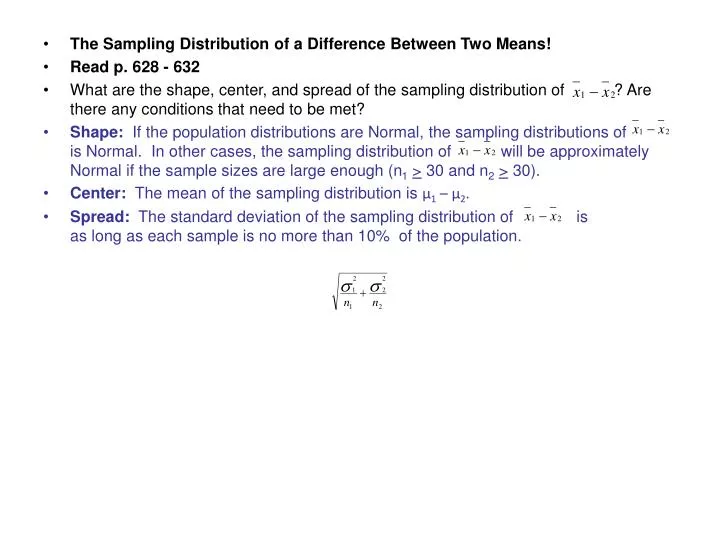
1. The Sampling Distribution of a Difference Between Two Means! • Read p. 628 - 632 • What are the shape, center, and spread of the sampling distribution of ? Are there any conditions that need to be met? • Shape: If the population distributions are Normal, the sampling distributions of is Normal. In other cases, the sampling distribution of will be approximately Normal if the sample sizes are large enough (n1> 30 and n2> 30). • Center: The mean of the sampling distribution is μ1 – μ2. • Spread: The standard deviation of the sampling distribution of is as long as each sample is no more than 10% of the population.

2. Example:" • A potato chip manufacturer buys potatoes from two different suppliers, Riderwood Farms and Camberley,Inc. The weights of potatoes from Riderwood Farms are approximately Normally distributed with a mean of 175 grams and a standard deviation of 25 grams. The weights of potatoes from Camberley are approximately • Normally distributed with a mean of 180 grams and a standard deviation of 30 grams. When shipments arrive at the factory, inspectors randomly select a sample of 20 potatoes from each shipment and weigh them. They are surprised when the average weight of the potatoes in the sample from Riderwood Farms is higher than the average weight of the potatoes in the sample from Camberley . • (a) Describe the shape, center, and spread of the sampling distribution of . • The shape of the sampling distribution of is approximately Normal since both population distributions are Normal. The mean of the sampling distribution is • 180-175=5 grams, and its standard deviation is • (b) Interpret the standard deviation of the sampling distribution of .

3. -3.7 5 13.7 -12.5 22.5 • (c) Find the probability that the mean weight of the Riderwood sample is larger than the mean weight of the Camberly sample. Should the inspectors have been surprised? • If the mean of the Riderwood sample is larger, then must be negative. The graph below shows the desired probability shaded. • The inspectors shouldn’t be surprised, because the Riderwood sample will have a higher mean more than one-fourth of the time.

4. The Two-Sample t Statistic! • Read p.633 - 634 • What is the standard error of ? Is this on the formula sheet? • The formula for standard deviation is but the formula • for standard error is not. • What is the formula for the two-sample t statistic? Is this one on the formula sheet? What does it measure? • No it is not. • It tells us how far is from its mean in standard • deviations units. • What distribution does the two-sample t statistic have? Why is this a t statistic rather than a z statistic? How do you calculate the degrees of freedom? • It has approximately a t distribution. Use is the t statistic when we don’t know the population standard deviation. • There are 2 ways. • 1) (technology) There is a some what messy formula. • 2) (conservative) Use the t distribution with degrees of freedom equal to the smaller of n1-1 and n2-1. With this option, the resulting confidence interval has a margin of error as large as or larger than is needed for desired confidence level. The significance test using this option gives a P-value greater of equal to the true P-value.

5. Confidence Intervals for μ1 - μ2! • Read p.634 - 637 • What are the conditions for a two-sample t interval for μ1 – μ2? • Random, Normal, Independent • What is the formula for the two-sample t interval for μ1 – μ2? Is this formula on the formula sheet? • This specific formula is not on the formula sheet, • but you are given the general formula for a confidence interval • and the formula for standard deviation of the sampling distribution. • Is it OK to use your calculator for the Do step? Are there any drawbacks? • It is ok to use your calculators. If you do, do not write the equation using conservative degrees of freedom. These will not produce the same answer. If you want to write out the formula, leave t* in the formula instead of putting in the conservative critical value. Then report the calculator’s interval and degrees of freedom.

6. Example: • Do plastic bags from Target or plastic bags from Bashas hold more weight? A group of AP Statistics students decided to investigate by filling a random sample of 5 bags from each store with common grocery items until the bags ripped. Then they weighed the contents of items in each bag to determine its capacity. Here are their results, in grams: • (a) Construct and interpret a 99% confidence interval for the difference in mean capacity of plastic grocery bags from Target and Bashas. • State: We want to estimate μT – μB at the 90% confidence level, where μT = the mean capacity of plastic bags from Target (in grams) and μB = the mean capacity of plastic bags from Bashas (in grams). • Plan: If the conditions are met, we will calculate a two-sample t interval for μT – μB. • Random: The students selected a random sample of bags from each store. • Normal: Since the sample sizes are small, we must graph the data to see if it is reasonable to assume that the population distributions are approximately Normal.

7. Since there is no skewness or outliers, it is safe to use t procedures. • Independent: The samples were selected independently, and it is reasonable to assume that there are at least 10(5) = 50 plastic grocery bags at each store. • Do: For these data, . Using a conservative df of 5-1=4, the critical value for 99% is t* = 4.604. The confidence interval is • With technology and df = 7.5, • CI = (-101, 7285) • Conclude: We are 99% confident that the interval from -1380 to 8564 grams captures the true difference in the mean capacity of plastic grocery bags from Target and from Bashas. • (b) Does your interval provide convincing evidence that there is a difference in the mean capacity between the two stores? • Since the interval includes 0, it is plausible that there is no difference in the two means. Thus, we do not have convincing evidence that there is a difference in mean capacity. However, if we increased the sample size, we would likely find a convincing difference since it seems pretty clear that Target bags have a bigger capacity.

8. Significance Tests for μ1 - μ2" • Read p. 638 - 643 • What are the conditions for conducting a two-sample t test for μ1 – μ2? • Random, Normal, and independent • Example: • In commercials for Bounty paper towels, the manufacturer claims that they are the “quicker picker-upper.” But are they also the stronger picker upper? Two AP Statistics students, Wesley and Maverick, decided to find out. They selected a random sample of 30 Bounty paper towels and a random sample of 30 generic paper towels and measured their strength when wet. To do this, they uniformly soaked each paper towel with 4 ounces of water, held two opposite edges of the paper towel, and counted how many quarters each paper towel could hold until ripping, alternating brands. Here are their results: • Bounty: 106, 111, 106, 120, 103, 112, 115, 125, 116, 120, 126, 125, 116, 117, 114 • 118, 126, 120, 115, 116, 121, 113, 111, 128, 124, 125, 127, 123, 115, 114 • Generic: 77, 103, 89, 79, 88, 86, 100, 90, 81, 84, 84, 96, 87, 79, 90 • 86, 88, 81, 91, 94, 90, 89, 85, 83, 89, 84, 90, 100, 94, 87 • (a) Display these distributions using parallel boxplots and briefly compare these distributions. Based only on the boxplots, discuss whether or not you think the mean for Bounty is significantly higher than the mean for the generic. • (b) Use a significance test to determine if there is convincing evidence that wet Bounty paper towels can hold more weight, on average, than wet generic paper towels.

9. a) Display these distributions using parallel boxplots and briefly compare these distributions. Based only on the boxplots, discuss whether or not you think the mean for Bounty is significantly higher than the mean for the generic. • The five-number summary for Bounty paper towels is (103, 114, 116.5, 124, 128), and the five-number summary for the generic paper towels is (77, 84, 88, 90, 103). Both distributions are roughly symmetric, but the generic brand has two high outliers. The center of the Bounty is much higher than the center of the generic distribution. Although the range of each distribution is roughly the same, the interquartilerange of the Bounty is larger. • Since the centers are so far apart and there is no overlap in the two distributions, the Bounty mean is almost certain to be significantly higher than the generic mean. If the true means were really the same, it would be virtually impossible to get so little overlap.

10. (b) Use a significance test to determine if there is convincing evidence that wet Bounty paper towels can hold more weight, on average, than wet generic paper towels. • State: We want to perform a test of H0: = µB - µG= 0 versus Ha: µB - µG > 0 at a 5% level of significance, where µB = the mean number of quarters a wet Bounty paper towel can hold and µG = the mean number of quarters a wet Generic paper towel can hold. • Plan: If the conditions are met, we will conduct a two-sample t test for µB - µG. • Random: The students used a random sample of paper towels. • Normal: Even though there are two outliers in the generic distribution, both distributions are reasonably symmetric, and the sample sizes are both at least 30, so it is safe to use t procedures. • Independent: The samples were selected independently, and it is reasonable to assume there are at least 10(30) = 300 paper towels of each brand. • Do: For these data, • test statistic: • P-value: Using either the conservative df = 30 – 1 = 29 or from technology, df = 57.8, the P-value is approximately 0. • Conclude: Since the P-value is less than 0.05, we reject H . There is very convincing evidence that wet Bounty paper towels can hold more weight, on average, than wet generic paper towels.

11. (c) Interpret the P-value from (b) in the context of this question. • Since the P-value is approximately 0, it is almost impossible to get a difference in means of at least 29.5 quarters by random chance if the two brands of paper towels can hold the same mean amount when wet. • Using Two-Sample t Procedures Wisely" • Read p. 644 - 648 • When doing two-sample t procedures, should we pool the data to estimate a common standard deviation? Is there any benefit? Are there any risks? • Do not pool the data for t procedures.  We DO have to pool when doing a significance test for the difference of 2 proportions but not with means. Should you use two-sample t procedures with paired data? Why not? How can you know which procedure to use? • Do not use these procedures with paired data because in paired data you arent looking for the difference between the means of the two groups - you are looking at the mean of the differences.  You determine which process to use by looking at the way the data is collected... Matched Pairs Experiment = Paired Data = one - sample t test Completely randomized experiment or stratified sampling = Difference of 2 Means = two-sample test

12. Example: • Suppose you are designing an experiment to determine if students perform better on tests when there are no distractions, such as a teacher talking on the phone. You have access to two classrooms and 30 volunteers who are willing to participate in your experiment. • (a) Design an experiment so that a two-sample t test would be the appropriate inference method. • On 15 index cards write “A” and on 15 index cards write “B”. Shuffle the cards and hand them out at random to 30 volunteers. All 30 subjects will take the same reading comprehension test. Subjects who receive A cards will go to a classroom with no distractions, and subjects who receive B cards will go to a classroom that will have the proctor talking on the phone during the test. At then end of the experiment, compare the mean score for subjects in room A with the mean score for subjects in room B. • (b) Design an experiment so that a paired t test would be the appropriate inference method. • Using the same procedure in part (a), divide the subjects into two rooms and give them the same reading comprehension test. One room will be distraction free, and the other room will have a proctor talking on the phone. Then, after a short break, give all 30 subjects a similar reading comprehension test but have the distraction in the opposite room. At the end of the experiment, calculate the difference in the two reading comprehension scores for each subject and c9ompare the mean difference with 0. • (c) Which experiment design is better? Explain. • The experiment design in part (b) is better since it eliminates an important source of variability – the reading comprehension skills of the individual subjects.