Download
1 / 12
130 likes | 278 Views
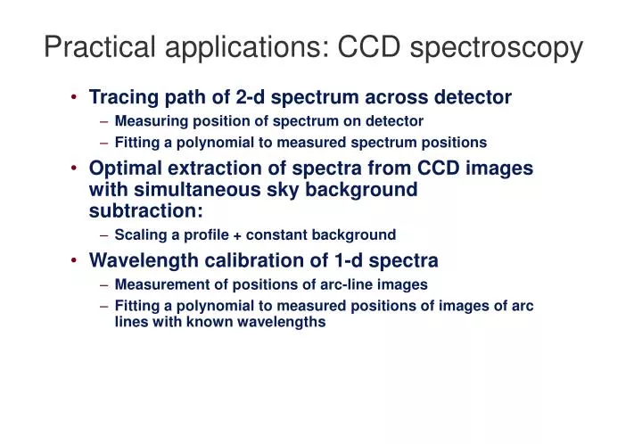
Practical applications: CCD spectroscopy. Tracing path of 2-d spectrum across detector Measuring position of spectrum on detector Fitting a polynomial to measured spectrum positions Optimal extraction of spectra from CCD images with simultaneous sky background subtraction:

E N D
Practical applications: CCD spectroscopy • Tracing path of 2-d spectrum across detector • Measuring position of spectrum on detector • Fitting a polynomial to measured spectrum positions • Optimal extraction of spectra from CCD images with simultaneous sky background subtraction: • Scaling a profile + constant background • Wavelength calibration of 1-d spectra • Measurement of positions of arc-line images • Fitting a polynomial to measured positions of images of arc lines with known wavelengths
x To zenith Target spectrum x (Reference spectrum) Night sky lines Observing hints • Rotate detector so that arc lines are parallel to columns: • To minimise slit losses due to differential refraction, rotate slit to “parallactic angle” • i.e. keep it vertical: • Spectra are then tilted or curved due to • camera distortions • Differential refraction
After bias subtraction and flat fielding • Recall Lecture 3 for subtraction of B(x,), construction of flat field F(x,) and measurement of gain factor G. • Corrected image values are
x x Tracing the spectrum • Spectra may be tilted, curved or S-distorted. • Trace spectrum via a sequence of operations: • divide into -blocks • measure centroid of spectrum in each block (fit gaussian) • fit polynomial in to calibrate x0(). • Once this is done, use x0() to select object/sky regions on subsequent steps. x0 x0
on edge of night-sky emission line Target Ref star x away from night-sky emission line Slices across spectrum at=const: Sky subtraction • Alignment (rotation) of CCD detector relative to grating aims to make ~const along columns. • Imperfect alignment gives slow change in along columns. • This causes gradient, curvature of sky background when is close to a night-sky line. • Solution: fit low-order polynomial in x to sky background data. • Alternative: fit linear function to interpolate sky from “sky regions” symmetric on either side of object spectrum: Target Ref
Slice across spectrum at =const: S(x) x x1 x2 “Normal” extraction • Subtract sky fit, and sum the counts between object limits: • Dilemma: How do we pick x1, x2? • too wide: too much noise • too narrow: lose counts
Slice across spectrum at =const: Starlight profile P(x) S(x) x x1 x2 Optimal extraction • 1) Scale profile to fit the data: • 2) Compute (x) from the model: • 3) -clip to “zap” cosmic-ray hits. • Iterate 1 to 3, since (x) depends on A:
Estimating the profile P(x) • The fraction of the starlight that falls in row x varies along the spectrum and is given by: • This is an unbiased but noisy estimator of P(x). • It varies as a slow function of wavelength. • Plot against and fit polynomials in at each x. Column 20 Column 60
Optimal vs. normal extraction • Pros: • Optimal extraction gives lower statistical noise. • Equivalent to longer exposure time • Incorporates cosmic-ray rejection • Cons: • Requires P(x,) slowly varying in (point sources). • Essential papers: • Horne, K., 1986. PASP 98, 609 • Marsh, T. and Horne, K.
Wavelength calibration • Select lines using peak threshold. • Measure pixel centroid xi by computing x or fitting a gaussian • Identify wavelengths i • Fit polynomial (x) to i, i=1,...,N. • Reject outliers (usually close blends) • Adjust order of polynomial to follow structure without too much “wiggling”. threshold level
Dealing with flexure • Flexure of spectrograph causes position xi of a given wavelength to drift with time. • Measure new arcs at every new telescope position. • Interpolate arcs taken every 1/2 to 1 hour when observing at same position. • Master arcfit: Use a long-exposure arc (or sum of many short arcs) to measure faint lines and fit high-order polynomial. • Then during night take short arcs to “tweak” the low-order polynomial coefficients.
Statistical issues raised • Outlier rejection: what causes outliers, and how do we deal with them? • Robust statistics. • Polynomial fitting: how many polynomial terms should we use? • Too few will under-fit the data. • Too many can introduce “flailing” at ends of range. • We’ll deal with these issues in the next lecture.